CDUNet: Cloud Detection UNet for Remote Sensing Imagery
←
→
Page content transcription
If your browser does not render page correctly, please read the page content below

remote sensing
Article
CDUNet: Cloud Detection UNet for Remote Sensing Imagery
Kai Hu        1,2     , Dongsheng Zhang 1 and Min Xia 1,2, *

                                          1   Collaborative Innovation Center on Atmospheric Environment and Equipment Technology, Nanjing
                                              University of Information Science and Technology, Nanjing 210044, China; 001600@nuist.edu.cn (K.H.);
                                              20201249164@nuist.edu.cn (D.Z.)
                                          2   Jiangsu Key Laboratory of Big Data Analysis Technology, Nanjing University of Information Science and
                                              Technology, Nanjing 210044, China
                                          *   Correspondence: xiamin@nuist.edu.cn

                                          Abstract: Cloud detection is a key step in the preprocessing of optical satellite remote sensing
                                          images. In the existing literature, cloud detection methods are roughly divided into threshold
                                          methods and deep-learning methods. Most of the traditional threshold methods are based on the
                                          spectral characteristics of clouds, so it is easy to lose the spatial location information in the high-
                                          reflection area, resulting in misclassification. Besides, due to the lack of generalization, the traditional
                                          deep-learning network also easily loses the details and spatial information if it is directly applied
                                          to cloud detection. In order to solve these problems, we propose a deep-learning model, Cloud
                                          Detection UNet (CDUNet), for cloud detection. The characteristics of the network are that it can
                                          refine the division boundary of the cloud layer and capture its spatial position information. In
                                          the proposed model, we introduced a High-frequency Feature Extractor (HFE) and a Multiscale
                                          Convolution (MSC) to refine the cloud boundary and predict fragmented clouds. Moreover, in order
                                to improve the accuracy of thin cloud detection, the Spatial Prior Self-Attention (SPSA) mechanism

                                          was introduced to establish the cloud spatial position information. Additionally, a dual-attention
Citation: Hu, K.; Zhang, D.; Xia, M.
                                          mechanism is proposed to reduce the proportion of redundant information in the model and improve
CDUNet: Cloud Detection UNet for
                                          the overall performance of the model. The experimental results showed that our model can cope
Remote Sensing Imagery. Remote Sens.
                                          with complex cloud cover scenes and has excellent performance on cloud datasets and SPARCS
2021, 13, 4533. https://doi.org/
10.3390/rs13224533
                                          datasets. Its segmentation accuracy is better than the existing methods, which is of great significance
                                          for cloud-detection-related work.
Academic Editors: Yang-Won Lee,
Jungho Im, Jaeil Cho and Chu-Yong         Keywords: cloud detection; cloud shadow; multiscale feature fusing; deep learning
Chung

Received: 30 September 2021
Accepted: 10 November 2021                1. Introduction
Published: 11 November 2021
                                               Pixel values indirectly reflect the spectral characteristics of ground objects, and differ-
                                          ent ground objects have different pixel values. Of course, excluding foreign objects with
Publisher’s Note: MDPI stays neutral
                                          the same spectrum, an important symbol to identify different ground objects in remote
with regard to jurisdictional claims in
                                          sensing image interpretation is the difference of the pixel values of the images. The pixel
published maps and institutional affil-
                                          value is also an important index reflecting the amount of information in an image.
iations.
                                               The traditional threshold method [1–3] excessively relies on artificial calibration based
                                          on pixel values, that is the characteristics of clouds—high reflection and low temperature—
                                          and distinguishes clouds from ground objects by analyzing their Nearinfrared Spec-
                                          trum (NIS). When it comes to complex situations, it is difficult to distinguish clouds
Copyright: © 2021 by the authors.         using these manually calibrated characteristics. For example, Kegelmeyer [1] used simple
Licensee MDPI, Basel, Switzerland.
                                          cloud pixels as the threshold. Although this method is simple and feasible, it often leads to
This article is an open access article
                                          the omission or misjudgment of cloud detection. Zhu et al. [2] proposed an object-oriented
distributed under the terms and
                                          Function of mask (Fmask) cloud detection method for remote sensing images captured
conditions of the Creative Commons
                                          by Landsat. This method uses cloud matching technology and a cloud height iterative
Attribution (CC BY) license (https://
                                          algorithm for cloud detection. Experience has proven that the overall accuracy of cloud
creativecommons.org/licenses/by/
                                          detection by the Fmask method is improved, but the detection rate of thin clouds is still not
4.0/).

Remote Sens. 2021, 13, 4533. https://doi.org/10.3390/rs13224533                                      https://www.mdpi.com/journal/remotesensing
Remote Sens. 2021, 13, 4533                                                                                         2 of 22

                              ideal. Candra et al. [3] added a Haze-Optimized Transformation (HOT) test and thermal
                              band in the previous multitemporal cloud masking algorithm to improve the algorithm
                              in the detection of haze, thin cirrus clouds, and thick clouds. They also improved the
                              previous multitemporal cloud masking in the detection of cloud shadow by adding a blue
                              band. Although their method is feasible and effective, the overall performance of cloud
                              segmentation is limited.
                                    With the rapid rise of deep learning, artificial neural networks are often used in
                              cloud detection research because of their good universality. This kind of method can
                              solve the problem of the temporal and spatial limitations of threshold methods to a great
                              extent by training datasets. The advantage of using deep learning to detect clouds is that
                              deep-learning models can automatically extract features from the images and complete
                              end-to-end training [4,5]; this automatic feature extraction based on convolution networks
                              provides higher accuracy for cloud and cloud shadow detection.
                                    In recent years, many methods based on deep learning have been proposed to detect
                              clouds, and multiscale feature fusion is often used in these methods. However, most
                              existing methods fuse features through concatenation and elementwise summation, which
                              are simple and can improve spatial information recovery. Besides, some cloud detection
                              results are not accurate enough near the boundary of clouds. In view of the above problems,
                              Wang et al. [6] proposed a cloud detection network, ABNet, which includes all-scale feature
                              fusion modules and a boundary point prediction module. The all-scale feature fusion mod-
                              ule can optimize the features and recover spatial information by integrating the features
                              of all scales. The boundary point prediction module further remedies cloud boundary
                              information by classifying the cloud boundary points separately. In addition, Xia et al. [7]
                              proposed a global attention fusion residual network method to segment clouds and cloud
                              shadow in satellite images. Meanwhile, the boundary refinement module was used to
                              predict the boundary of clouds and shadows, so as to refine the boundary information.
                                    Cloud and shadow segmentation is more challenging when only a limited number of
                              spectral bands are available. To solve this problem, Mohajerani et al. (2019) [8] proposed
                              an algorithm based on deep learning. The algorithm consists of a fully convolutional
                              network [9], which is trained from multiple patches of Landsat 8 images. This network,
                              known as cloud-net, is capable of capturing global and local cloud features in images using
                              convolutional blocks.
                                    Cloud and snow detection has significant remote sensing applications, while clouds
                              and snow share similar low-level features due to their consistent color distributions and
                              similar local texture patterns. Thus, accurately distinguishing clouds from snow at the
                              pixel level from satellite images is always a challenging task with traditional approaches.
                              To solve this shortcoming, Zhan et al. (2017) [10] proposed a deep-learning system for
                              cloud and snow classification based on a pixel-level fully convolutional neural network
                              using satellite images in three visible bands.
                                    In addition, Dronner et al. [11] used the FCN architecture to detect clouds in mul-
                              tispectral remote sensing images. However, in the FCN framework, as it ignores the
                              high-resolution feature image, the edge information is lost, so the segmentation results are
                              poor in detail. Chai et al. [12] proposed a codec-based adaptive SegNet [13] for cloud and
                              cloud shadow detection in Landsat images. However, SegNet has an insufficient grasp on
                              the global semantic information and often makes misjudgments. Ronneberger et al. [14]
                              proposed the U-shaped network (UNet), which can capture multiscale semantic informa-
                              tion through repeated downsampling and upsampling of the deep network. However, due
                              to the irregular geometry of clouds, it easily ignores the boundary information of fuzzy
                              objects such as thin clouds:
                              •    The location of clouds is often complex and diverse, and the distribution of clouds is
                                   often irregular and discontinuous. The traditional threshold method usually needs to
                                   use experience and manual calibration, so the prediction accuracy and universality
                                   are poor. Besides, the existing neural networks have defects in global information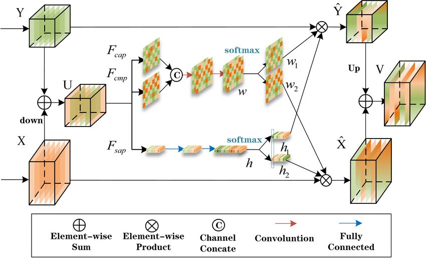
Remote Sens. 2021, 13, 4533                                                                                            3 of 22

                                   extraction, which easily lose the relative position information between clouds and
                                   shadows, so they easily cause category error detection;
                              •    Cloud boundaries are often irregular geometric features. Therefore, we paid more
                                   attention to the prediction of cloud boundaries during model training. We hoped to
                                   complete the alignment directly in the end-to-end training process without the help of
                                   boundary postprocessing.
                                   In view of the above findings, we propose a U-shaped structure model based on the
                              deep-learning method, which uses ResNet [15] as the backbone network. ResNet joins
                              the residual unit through a short-circuit mechanism. Because of its simple structure and
                              excellent performance, it is often used as the backbone of segmented networks. The key to
                              the performance of the U-shaped structure lies in the feature fusion stage. In the feature
                              fusion stage, we used a High-frequency Feature Extractor (HFE) for the shallow input
                              to extract the high-frequency information of the image, and at the same time, we used
                              the Multiscale Convolution (MSC) to filter out the unnecessary high-frequency signal, so
                              as to optimize the edge of the cloud. For the deep input, we integrated the Spatial Prior
                              Self-Attention (SPSA) to obtain distance information between classes, so as to strengthen
                              the control of global information and make the model have better spatial adaptability. In
                              addition, we also introduced the Spatial Channel Attention Block (SCAB) to reduce the
                              proportion of redundant information in the feature map and improve the efficiency of cloud
                              detection. Finally, our model achieved a 93.52% Mean Intersection over Union (MIoU) on
                              the three cloud and cloud shadow classification datasets and showed the highest perfor-
                              mance. In order to verify the generalization of the model, we also conducted experiments
                              on the Star-Planet Activity Research CubeSat (SPARCS) dataset. The experimental results
                              showed that our model is also ahead of the existing CNN model and can complete the
                              cloud and cloud shadow segmentation tasks well. In summary, our research contributions
                              are as follows:
                              •   The traditional segmentation network will lose a portion of the detailed information
                                  in the downsampling stage. In order to refine the edge, we designed a high-frequency
                                  feature extractor to extract the detailed information of the image; convolution proved
                                  to be an effective feature extraction tool, and it also can be regarded as a special filter,
                                  so we designed a Multiscale Convolution module (MSC) to “filter” the image. While
                                  suppressing high-frequency noise, it extracts effective texture information, which can
                                  make the model predict more refined edges;
                              •   The deep feature map contains lower-frequency signals, having stronger intraclass
                                  consistency, but weakening the interclass information. In order to re-establish inter-
                                  class information, we designed a Spatial Prior Self-Attention block (SPSA) for the
                                  convolution neural network, which can better distinguish cloud, cloud shadow, and
                                  background information;
                              •   A segmentation network based on an encoder–decoder will inevitably produce se-
                                  mantic dilution in the feature fusion stage. Other studies [14,16–18] simply combined
                                  high-level context information with Low-level spatial information to solve the above
                                  problems. This easily produces information redundancy, and consequently, the convo-
                                  lution kernel cannot receive effective feature information. In our method, we designed
                                  a parallel Channel Spatial Attention Block (SCAB) in the feature fusion stage, so
                                  that the model can quickly capture effective information and improve the prediction
                                  accuracy.

                              2. Methodology
                                   Based on the above discussion, the semantic segmentation cloud detection model still
                              needs improvement in the detail feature extraction and upsampling feature fusion stages.
                              In this part, we first introduce the architecture of Cloud Detection UNet (CDUNet) and,
                              then, focus on the feature fusion layer and its submodules: HFE, MSC, SPSA, and SCAB.
Remote Sens. 2021, 13, 4533 4 of 22
2.1. Network Architecture
The accuracy of feature extraction directly affects the accuracy of the final classifica-
tion [19,20]. Each layer of ResNet contains different levels of semantic information, which
help us quickly extract multiscale information, and the residual structure of ResNet helps
solve the problem of the gradient explosion and the vanishing gradient caused by the
deepening of the network. Therefore, we used ResNet as the backbone network for remote
sensing image segmentation. In addition, Lin et al. [21] proved that a 1 × 1 convolution can
be used to change the number of channels, that is dimensionality reduction and increased
information. The amount of calculation caused by the segmentation task is huge, and at the
same time, to ensure the model’s performance, we did not reduce the number of channels
in the encoding stage, but used a 1 × 1 convolution in the decoder stage to reduce the
number of channels to 1/2 of the original, thereby reducing the overall parameters of the
model. The overall structure is shown in Figure 1.
Figure 1. Framework of the proposed CDUNet. The framework is mainly composed of three parts: encoder, decoder, and
booster. In the encoder stage, ResNet50 is responsible for extracting the semantic information; in the decoder stage, decoding
information is extracted from the upsampling interaction layer; finally, the booster stage accelerates the segmentation
efficiency and summarizes the information of each layer to complete the segmentation task.
In the decoder stage, the existing network cannot recover the lost details effectively.
In order to solve this problem, we designed a feature fusion layer, which is also the most
important part of CDUNet. As shown in Figure 2a,b, this layer is composed of the HFE,
MSC, SPSA, and SCAB modules. As for the network function, the HFE module is mainly
used to recover the details lost in the encoder stage; the MSC module is used to extract
the multiscale information existing in the channel; the SPSA module is used to reconstruct
the spatial location information from the deep network in the decoding stage; the SCAB
module is used to improve the information redundancy in the feature map. From the
aspect of the network structure, this layer is composed of two branches, one of which is a
relatively high-resolution feature map generated from the shallow branch, and the other
is a relatively low-resolution feature map with rich background information extracted
through multiple downsampling operations. The two branches interact with the semantic
information before entering the SCAB module. Each layer of the high-resolution and
low-resolution representations receives information repeatedly, thus reducing the loss
of semantic information and obtaining relatively rich feature representations. As shown
in Figure 2c, Seg Head is a unique module of CDUNet in the training stage, which is
composed of a convolution layer and a dropout layer. Its function is to speed up the
convergence of the network and improve the prediction accuracy.Remote Sens. 2021, 13, 4533 5 of 22
(a) (b) (c)
Figure 2. Proposed CDUNet structure: (a) Detail structure of Fuse Layer 1. (b) Detail structure of
Fuse Layers 2–4. (c) Seg Head. ⊕ means elementwise add.
2.2. High-Frequency Feature Extractor
From the basic model of deep learning, LENet5, Reference [22] used the downsampling
operation to reduce the information dimensionality, and the downsampling operation
played a role in reducing the computational complexity and expanding the receptive
field. At the same time, the low-pass filtering effect brought by the subsampling operation
on the image is irreversible. In order to reproduce this part of the lost high-frequency
information, we designed an HFE. In the encoder process, the classic network UNet [14]
draws a semantic branch from each layer and passes it from the encoder to the decoder of
the same number of layers through the concatenate operation, thereby introducing high-
resolution information, which can provide relatively fine features for segmentation, such as
the edge of an object, etc. Our model continues this idea and introduces a high-frequency
extractor to refine the high-resolution information brought by the shallow layer of the
network. The method we used is to derive a branch from each layer of ResNet. This branch
has not the undergone downsampling and convolution operations for the current layer, so
it has rich semantic information. The details are shown in Figure 3. Its structure is simple
and clear. Firstly, its input comes from two parts: one of them is from the shallow layer of
the network, and the other is from the deep layer of the network. These two parts contain
different characteristic information. Under ideal conditions, we believe that the former
contains more information than the latter, or that the latter is a subset of the former. We
make a convolution operation and upsampling operation on the deep feature map, enlarge
it to the same size as the shallow feature map, and then subtract them. In this way, we
obtain the relatively high-frequency feature map. Although the high-frequency signal is
effective, it also has noise, so we set a learnable parameter to make the network adjust
the proportion of the high-frequency signal independently. In this module, an addition
operation is used to superimpose our high-frequency feature map on the original feature
map to enhance the high frequency.Remote Sens. 2021, 13, 4533 6 of 22
Figure 3. The structure of the high-frequency feature exacter, where ⊕, represent elementwise add
and subtract, respectively.
The design purpose of the module is to make up for the signal loss caused by the
downsampling. The above steps can be expressed as follows:
F̂y = up (δ ( Fy ) ) , Fy ∈ Rh/2×w/2×c/2 , F̂y ∈ Rh×w×c , (1)
Fh = Fx − F̂y , Fx ∈ Rh×w×c , Fh ∈ Rh×w×c , (2)
F̂x = Fx + γ × Fh , Fh ∈ R H ×W ×C , (3)
where R represents the real number field, h, w, c represent the height, width, and channel
number of the feature graph, respectively, Fx represents the shallow input, Fy is the deep
input, δ (·) means the convolution operation is used to unify the number of channels, up (·)
means the upsampling operation is used to unify the size of the feature map, F̂y is the deep
input after the upsampling and amplification, Fh is the high-frequency characteristic map
obtained by subtracting Fx and F̂y , γ represents the weight coefficient, and F̂x is the final
feature map after the high-frequency enhancement.
In order to verify the effectiveness of the module, we input three test images and
used the heat map to represent the stage feature map. Figure 4b represents the shallow
input, while Figure 4c,d represents the deep input and the high-frequency characteristic
graph obtained by the subtraction operation. Not surprisingly, we found that with the
supplement of the shallow feature map, the final output feature map in Figure 4e has more
abundant texture information. This shows that the HFE module effectively extracted the
high-frequency features, and it was more accurate for the cloud and shadow location and
the boundary prediction.Remote Sens. 2021, 13, 4533 7 of 22
(a) (b) (c) (d) (e)
Figure 4. Heat map representation. (a) Test image; (b) shallow features; (c) deep features; (d) high-
frequency features; (e) output features. The above images are from the cloud and cloud
shadow datasets.
2.3. Multiscale Convolution
Although the HFE can extract the high-frequency information of the image, such
as the boundary of the cloud layer and the sparse distribution of the point cloud, at the
same time, noise is inevitably introduced, so we wanted to use a convolution layer to
further filter the information. Representing features on multiple scales is very important
for many visual tasks, and the majority of existing methods [23–25] represent multiscale
features in a hierarchical way. We hoped to construct hierarchical residual class connections
within a single residual block to represent multiscale features in a more fine-grained way
and increase the receptive field of each network layer. In order to achieve the above
functions, we designed an MSC module to filter the high-resolution feature map after the
high-frequency extractor and further extract the multiscale features of the feature map.
As shown in Figure 5, except for the normal 3 × 3 convolution, we introduced a set
of convolutions with kernel sizes of 5 × 5 and 7 × 7 to expand the receptive field and
enrich the multiscale information. In order to reduce the number of parameters of the
model, this design used the split method to perform the 5 × 5 and 7 × 7 convolutions in
a parallel cascade, which has the same receptive field as the original convolution kernel.
Due to the combination effect, many equivalent feature scales are generated. This structure
can enhance the feature selection ability of the convolution kernel from the scale level.
Specifically, the MSC first accepts the high-frequency fusion features from the HFE module.
After a 1 × 1 convolution, we evenly divided the feature map Fin into s feature map subsets,
denoted by xi , i ∈ {1, 2, · · · , s}. Each feature subset had the same size as the original feature
map, but the number of channels was reduced to the original 1s . Other features except x6
had a corresponding convolution layer, and the corresponding convolution operation is
shown by Ci (·) , so the output yi of each layer can be expressed by the following formula:
Ci ( xi ) , i = 1
yi = Ci ( xi + yi−1 ), 1 < i < s. (4)
xi , i = s
Remote Sens. 2021, 13, 4533                                                                                            8 of 22

                              Figure 5. Multiscale convolution block.

                                   After that, we merged the channels of each yi and then through the 1 × 1 convolution,
                              with the introduction of the residual structure. Finally, we obtained the desired feature map.
                              In order to enhance the feature extraction ability, we reused two layers of the multiscaling
                              in the feature fusion stage, and the details can be seen in Figure 2.

                              2.4. Spatial Prior Self-Attention
                                    The work of Luo et al. [26] showed that the receptive field acted on by the convolution
                              kernel is local and can only be correlated with the regions of different parts of the whole
                              image after accumulating through many layers; that is because deep feature maps often
                              contain more low-frequency signals, which have stronger intraclass consistency. When we
                              consider the local feature aggregation of a pixel, we should pay attention to those pixels that
                              have a greater impact on it. Therefore, we propose a spatial prior self-attention mechanism.
                              This module uses the vector dot product to establish spatial location information between
                              pixels, so that clouds and cloud shadows can be connected to the surrounding ground
                              object information, so as to better distinguish the ground object information.
                                    The nonlocal attention mechanism [27] proposed by Wang et al. uses vector dot multi-
                              plication to establish the spatial position relationship, but it takes up additional memory
                              capacity, which is very unfriendly to the training process. DANet [28] attaches two types
                              of attention modules to the backbone network to simulate the semantic interdependence in
                              the space and channel dimensions, respectively; at the same time, DANet occupies much
                              memory capacity. CCNet [29] obtains the pixel-level position information through the
                              cross-path of each pixel, and then, through a circular operation, each pixel can capture the
                              whole image dependency of all pixels. This cross-calculation method reduces the amount of
                              calculation by losing a small amount of performance. As shown in Figure 6, we introduced
                              an SPSA module to solve this problem. The difference from the above self-attention module
                              is that we embedded two learnable vectors into the K vector, which is regarded as the
                              horizontal and vertical spatial attention, which is equivalent to the introduction of a spatial
                              prior. Ph and Pw represent the priors of the spatial position in the H and W dimensions
                              respectively, which are a group of learnable vectors. They can update the gradients in the
                              backpropagation, so as to optimize the pixels in the H and W dimensions and obtain the
                              spatial attention map. The calculation formula is as follows:
Remote Sens. 2021, 13, 4533 9 of 22
θ̂ ( xi ) = BNγ,β (Wθ xi ), (5)
φ̂ ( x j ) = BNγ,β (Wφ x j ), (6)
ĝ ( x j ) = BNγ,β (Wg x j ), (7)
1 T
Z = softmax ( (K + P) T Q) V + X = T
e (θ̂ ( xi ) + pw + ph ) φ̂ ( x j )
ĝ ( x j ) + ∑∀ xi , (8)
(θ̂ ( xi ) + pw + ph ) φ̂ ( x j ) i
∑∀ j e
where Q, K, and V represent the query, key, and value, respectively, P is the prior of spatial
position, X represents the input feature map, xi represents the information of the current
focus location, x j represents the global information, θ̂ (·) , φ̂ (·) , and ĝ (·) respectively
represent the 1 × 1 convolution and batch normalization operations. The final output is
represented by Z. In addition, in order to reduce the amount of calculation, we adjusted
the channel dimensions. We reduced the dimensions of the k vector, the q vector, and Pw
and Ph in the channel dimension. Considering the amount of calculation, this module is
only used on the low-resolution side of the feature fusion layer, and in order to improve
the performance of the model in the feature fusion stage, we repeatedly used the SPSA
module twice.
Figure 6. Spatial prior self-attention block. BN represents the Batch Normalization layer.
2.5. Spatial Channel Attention Block
In the feature fusion stage, the encoder–decoder-based segmentation network will
inevitably produce semantic dilution, and most of these networks adopt simple feature
graph addition or channel merge operations, which easily produce information redundancy,
so that the convolution kernel cannot receive effective feature information. Inspired by
Li et al. [30] and Woo et al. [31], in order to effectively integrate multilevel/multiscale
feature maps, we designed a parallel spatial channel attention mechanism in the feature
fusion stage, so as to enable the model to quickly capture effective information and improve
the prediction accuracy.
As shown in Figure 7, we used the cross-branch relationship between the two input
branch feature maps to generate spatial channel attention weights; that is, feature map
X ∈ Rh×w×c is downsampled and added to feature map Y ∈ Rh/2×w/2×c to form attention
map U ∈ Rh×w×c . The maximum pooling and average pooling operations are used to
generate the spatial attention map, and then, two layers of convolution are used to extract
the spatial information.Remote Sens. 2021, 13, 4533 10 of 22
Figure 7. Spatial channel attention block.
The final spatial attention map w ∈ Rh×w×2 can be expressed by the following formula:
Xi
U =Y+ ∑ s2
, (9)
i ∈h×w
w = f 1×7 ( f 7×1 ( Fcap (U ) ; Fcmp (U ) ) ),
(10)
where s represents the downsampling step size, which was set to two here; Fcap (·) and
Fcap (·) are the global average pooling and global maximum pooling for aggregating
channel information; f 1×7 and f 7×1 represent the 1 × 7 and 7 × 1 convolution operations,
respectively. Similarly, we used the average pooling to generate channel feature e ∈ R1×1×c
in the spatial dimension of U ∈ Rh×w×c and, then, used two fully connected layers to
extract the channel information, so that the channel attention map h ∈ 1×1×2c can be
expressed by the following formula:
h = f f c1 ( f f c0 ( Fsap (U ) ) ), (11)
Fsap (·) is the global average pooling for aggregating spatial information. f f c1 and f f c0
represent the full connection layer. Then, we used the softmax operation for the spatial
attention map and channel attention map to obtain the spatial and channel attention
weights, that is:
( w1 ; w2 ) = σ ( w ) , (12)
( h1 ; h2 ) = σ ( h ), (13)
where σ (·) is the softmax operator, w1 ∈ Rh×w and w2 ∈ Rh×w represent the spatial
weights of Y and X, respectively, and h1 ∈ Rc and h2 ∈ Rc represent the channel weights of
Y and X, respectively. The high and low resolution features Ŷ ∈ Rh×w×c , X̂ ∈ Rh/2×w/2×c
and the final fusion feature V ∈ Rh×w×c can be calculated as follows:
Ŷ = w1 ⊗ Y + h1 ⊗ Y, (14)
X̂ = w2 ⊗ X + h2 ⊗ X, (15)
V = up (Ŷ ) + X̂, (16)
where ⊗ a is the matrix multiplication and up (·) is the two-times upsampling. Finally, we
obtained the feature map optimized by the spatial channel attention.Remote Sens. 2021, 13, 4533 11 of 22
As shown in Figure 8, we added the attention map to the original image to obtain the
above images. From the graph, we can see that after adding the channel space attention
model, our model will pay more attention to the effective information of the network
prediction and make the prediction target clearer.
(a) (b) (c)
Figure 8. Heat map representation. (a) Test image; (b) model without the SCAB; (c) model with the
SCAB. The above images are from the cloud and cloud shadow datasets.
3. Experiment
3.1. Dataset Introduction
3.1.1. Cloud and Cloud Shadow Dataset
The cloud and cloud shadow datasets used in this paper were from Google Earth,
which is a virtual Earth software developed by Google. It puts satellite photos, aerial photos,
and the GIS on the 3D model of the Earth. The effective resolution of global geomorphologic
images on Google Earth is at least 100 m, usually 30 m (for example, Mainland Chinese), and
the altitude of the view (Eyealt) is 15 km. The dataset is composed of high-definition remote
sensing images randomly collected by professional meteorological experts in Qinghai,
the Yunnan Plateau, the Qinghai Plateau, the Qinghai Tibet Plateau, and the Yangtze
River Delta. In order to better reflect the performance of the model, we selected several
groups of high-resolution cloud images with different shooting angles and heights. Due
to the limitation of the GPU video memory capacity, we cut the high-definition cloud
remote sensing image with the original resolution of 4800 × 2692 to a size of 224 × 224.
After screening, we obtained a total of 9217 images, among which 7374 were used as the
training set and 1843 as the verification set. The ratio of the training set to the verification
set in the dataset was 8/2. As shown in Figure 9, the high-resolution cloud and cloud
shadow images derived from Google Earth are roughly divided into 5 types, which have
different backgrounds, namely water area, woodland, farmland, city, and desert. The tags
are manually tagged and come in three types: cloud (red), cloud shadow (green), and
background (black).Remote Sens. 2021, 13, 4533 12 of 22
(a) (b) (c) (d) (e)
Figure 9. Display of some of the training data. (a) Water area; (b) woodland; (c) farmland;
(d) cities; (e) desert.
3.1.2. SPARCS Dataset
The SPARCS dataset was collected from the Landsat 8 satellite, which includes two
types of sensors: Operational Land Imager (OLI) and Thermal Infrared Sensor (TIRS). The
band information is shown in Table 1. The SPARCS dataset [32,33] was originally created
by M. Joseph Hughes of Oregon State University and manually exported from Landsat
8 OLI scenarios. Its purpose is to verify cloud and cloud shadow masking derived from
the Spatial Program for Automatic Cloud and Shadow Removal (SPARCS) algorithm. The
cloud validation dataset contains 80 subsets of 1000 × 1000 px scenarios, including cloud,
cloud shadow, snow/ice, waters, and background. Limited by the video memory capacity
as well, we cut the original dataset into 256 × 256 px and obtained a total of 1280 images.
We divided the dataset into a training set and a verification set at a ratio of 8/2. Due to
the small size the original datasets, overfitting was prone to occur. In order to enhance the
generalization ability of the model, we expanded the datasets by horizontal flipping (50%),
vertical flipping (50%), and random rotation (−30°∼30°, 50%) and finally obtained 2534
training sets and 634 verification sets.
Table 1. Spectral bands for the Landsat 8 sensors.
Landsat 8
Band Wavelength (nm) Resolution (m)
1 (Coastal) 430–450 30
2 (Blue) 450–515 30
3 (Green) 525–600 30
4 (Red) 630–680 30
5 (NIR) 845–885 30
6 (SWIR-1) 1560–1660 30
7 (SWIR-2) 2100–2300 30
8 (PAN) 503–676 15
3.2. Training Detail
Our experimental implementation was based on the public platform PyTorch (Version:
0.40) (Paszke et al. 2017) [34]. In this work, we used the “Steplr” learning rate strategy,
epoch
that is lrnew = lrinitial × γ stepsize , setting the baseline learning rate as 0.001, the adjustment
multiple as 0.95, and the adjustment interval as 3. A total of 200 iterations were carried
out, and the cross-entropy was used as the maximum loss function. Because the Adam
optimizer [35] converges quickly and stably, in the experiments involved in this article,
we use Adam as the optimizer, where β 1 was set to 0.9 and β 2 to 0.999. Our training
device uses the NVIDIA GeForce RTX 3080 with a video memory capacity of 10 G, whichRemote Sens. 2021, 13, 4533 13 of 22
is limited by the physical memory of a single GPU. When training the cloud and cloud
shadow datasets, we set the batch size to 16, and when training the SPARCS dataset, we
set the batch size to 6.
In addition, we also selected the parameters of the backbone network ResNet before
the comparison experiment and ablation experiment. Three groups of comparison experi-
ments were conducted on the cloud and cloud shadow dataset, namely Resnet34, Resnet50,
and Resnet101. Through the experiments, we found that the model using Resnet50 as
the backbone network had the highest MIoU, indicating that Resnet50 with a moderate
number of parameters was more suitable for subsequent experiments in the case of a small
number of categories. See Table 2 for the relevant experiments.
Table 2. Selection of the backbone network.
Method PA (%) MIoU (%) Parameter (M) Flops (G)
ResNet34 96.49 91.83 21.99 3.82
ResNet50 96.68 92.28 34.49 5.63
ResNet101 96.50 91.85 53.48 9.34
3.3. Loss Function
Inspired by Hengshuang Zhao et al.’s setting of auxiliary loss in the pyramid scene
parsing network [36], this paper also set the auxiliary loss and main loss to supervise the
learning. When a network is deep, the introduction of auxiliary loss helps to optimize the
learning process without affecting the learning of the main branch. In order to facilitate pa-
rameter adjustment, we introduced a total of four layers of semantic headers (see Figure 1).
In the experiment, in order to ensure the fairness of the experiment, including the main loss,
the weight coefficients of the two datasets were set as 1:1:1:1. In practical applications, the
auxiliary loss of this model can be adjusted according to the actual situation. In addition,
in order to avoid overfitting, we introduced a regularization term to the loss function.
Therefore, the final loss function is defined as:
4
λ5
L ( Θ ) = λ1 L p ( Θ ) + ∑ λ i L ai ( Θ ) + k Θ k2 , (17)
i =2
2
where L p is the principal loss, L a is the auxiliary loss, the λ1 –λ5 ratio is set to 1, and the
network parameter Θ is updated through iterations to minimize the final loss L (Θ) .
The experimental results are shown in Table 3. After the auxiliary loss was added, its
parameters increase slightly, but the PA (%) and MIoU (%) were 0.13% and 0.34% higher
than the benchmark network.
Table 3. Setting the booster with auxiliary loss.
Method Booster PA (%) MIoU (%) Parameter (M)
ResNet50 × 96.55 91.94 33.97
ResNet50 X 96.68 92.28 34.49
3.4. Ablation Study
The fuse layer was composed of four components: HFE, MSC, SPSA, and SCAB.
Table 4 compares the improvement of the network prediction accuracy of each module
and gives the parameters and calculation amount of the model. We performed an ablation
study using the cloud and cloud shadow datasets:
• Ablation for the HFE: The existing network can easily lose high-frequency information
during the coding stage because of the sampling operation. The high-frequency feature
extractor can recover some high-frequency components in the feature map. These
high-frequency components include the texture characteristics of the cloud, which
have a positive effect on the prediction of the results. As shown in Table 4, the HFERemote Sens. 2021, 13, 4533 14 of 22
can increase the MIoU of the model from 92.28% to 92.56% and the PA from 96.68% to
96.81% due to the reappearance of details;
• Ablation for MSC: After high-frequency feature enhancement, the feature maps ob-
tain more information, and multiscale convolution can extract effective multiscale
information from them. As can be seen from the results in Table 4, the MSC module
improved the MIoU of the model by 0.2% and the PA by 0.1%;
• Ablation for SPSA: The space prior self-control module can establish the position
relationship between pixels, so that classification information can greatly improve the
prediction accuracy. However, at the same time, the parameter and calculation amount
brought by the module are huge. MobileNet determines the influence of network
width on performance [37]. The study showed that there is redundancy in the feature
graph channel, which can reduce the redundancy through the compression channel,
and the number of overcompressed channels will also make the information that the
network can capture limited. In order to filter the redundant channel information
better and reduce the parameter quantity, we suggest that the channel reduction ratio
R be greater than or equal to 2. As shown in Table 5, we found that when r = 4, the
performance was the best, and the parameters and the number of calculations were
relatively appropriate. In addition, we added the ablation experiment of the Pw and
Ph priors. The experimental comparison results in Table 6 showed that the model
with the Pw and Ph priors had the best performance, which also explained how the
introduction of learnable parameters help extract the spatial information from the
model;
• Ablation for the SCAB: The feature map extracted by the multiscale module has six
groups of multiscale information of different receptive fields, but the weights of this
information with respect to the prediction results are different; the SPSA module
establishes the location information of the feature map pixels, but ignores the channel
information. Therefore, we hoped to reduce the redundancy of multiscale information
by adjusting the channel weight and spatial weight of the feature map and strengthen
the spatial location information to highlight the key points. Through the experiment,
the MIoU of our model improved to 93.52%, and the PA improved to 97.22%.
Table 4. The performance comparison of the networks using the proposed modules (bold represents the best result).
Method PA (%) MIoU (%) Parameter (M) Flops (G)
ResNet50 96.68 92.28 34.49 5.63
ResNet50 + HFE 96.81 92.56 35.19 5.74
ResNet50 + HFE + MSC 96.91 92.76 39.06 7.54
ResNet50 + HFE + MSC + SPSA 97.14 93.36 46.55 8.4518
ResNet50 + HFE + MSC + SPSA + SCAB 97.22 93.52 47.59 8.4520
Table 5. The performance comparison of SPSA with different reduction rates (bold represents the
best result).
Reduction Rate PA (%) MIoU (%) Parameter (M) Flops (G)
2 97.11 93.27 47.95 8.61
4 97.14 93.36 46.55 8.45
6 97.09 93.22 45.85 8.37
8 97.09 93.17 45.50 8.34Remote Sens. 2021, 13, 4533 15 of 22
Table 6. The performance comparison of the self-attention modules (- represents no self-attention
modules; bold represents the best result).
Method PA (%) MIoU (%) Parameter (M) Flops (G)
- 97.04 93.08 43.43 7.99
SA 97.15 93.36 47.57 8.44
SPSA 97.22 93.52 47.59 8.45
3.5. Comparison Test of the Cloud and Cloud Shadow Datasets
In this section, we compare the proposed method with other semantic segmenta-
tion networks. In this paper, the Pixel Accuracy (PA), Mean Pixel Accuracy (MPA), F1-
score, Frequency-Weighted Intersection over Union (FWIoU), and Mean Intersection over
Union (MIoU) were selected as the evaluation results of the experimental results. The
quantitative results of the above indicators are listed in Table 7. CDUNet had the best
results among all the competitive methods. By loading the pretrained model [38] on the
backbone network, our network was also ahead of other models in various indicators,
which shows the effectiveness of our proposed method.
Due to the space limitations, it is not possible to show the effect drawings of all
models, so the six models with higher indicators and strong representation were selected
for Figure 10. Because PSPNet and CCNet use a pyramid pooling module and a crisscross
attention module, respectively, they are more dominant in the global receptive field. How-
ever, the details of the above two networks, such as the boundary of the cloud layer and
the point cloud fragments, can not be well predicted. This is because PSPNet and CCNet
lose much detail information after repeated downsampling, so they are not dominant in
the presentation of cloud detail information. It can be seen from the figure that under
the background of desert, water area, and forest land, the single-path models PSPnet and
CCNet can only predict the general outline of clouds and cloud shadows, while multi-
branch networks such as HRNet and CloudNet retain some details, so the prediction of
the cloud edge is more accurate. It can be observed that in the complex background, the
high-frequency feature extractor designed by us fully retained the high-frequency infor-
mation lost in the downsampling process, which contains rich details. At the same time,
the multiscale convolution designed by us had a filtering role and filtered out unnecessary
high-frequency noise. Therefore, our model can preserve the detail information to a great
extent and can also completely preserve the shape and boundary of clouds and cloud
shadows, which further proves the effectiveness of the proposed method.
Table 7. Results on the cloud and cloud shadow datasets. Pretrained methods are marked with
“† ” (bold represents the best result).
Method PA (%) MPA (%) F1 (%) FWIoU (%) MIoU (%)
SegNet [13] 94.86 93.96 90.72 90.26 88.18
BiSeNetv2 [39] 95.75 94.95 92.35 91.88 90.17
DenseASPP [40] 95.99 94.44 93.11 92.35 90.65
FCN8s [11] 96.00 94.92 92.91 92.35 90.69
DeepLabv3+ [41] 96.17 95.32 93.11 92.66 91.06
UNet 96.27 95.39 93.32 92.83 91.29
GAFRNet [7] 96.30 95.50 93.40 92.90 91.41
CloudNet [8] 96.37 95.61 93.44 93.01 91.51
PSPNet 96.53 95.86 93.79 93.33 91.88
CCNet 96.58 95.70 93.94 93.42 92.02
HRNet [42] 96.61 95.78 93.95 93.47 92.06
Ours 97.22 96.60 95.07 94.61 93.52
FCN8s † 97.02 96.60 94.52 94.22 92.99
CCNet † 97.13 96.44 94.88 94.43 93.26
PSPNet † 97.17 96.43 94.96 94.51 93.34
Ours † 97.51 96.89 95.56 95.15 94.12Remote Sens. 2021, 13, 4533 16 of 22
(a) Image (b) Label (c) GAFRNet (d) CloudNet (e) PSPNet (f) CCNet (g) HRNet (h) CDUNet
Figure 10. The prediction results of a set of test pictures. (a) The original images; (b) corresponding labels; (c) the predicted
maps of GAFRNet; (d) the predicted maps of CloudNet; (e) the predicted maps of PSPNet; (f) the predicted maps of
CCNet; (g) the predicted maps of HRNet; (h) the predicted maps of CDUNet.
Figure 11 shows the visual effects of different methods on cloud and cloud shadow
images. The extraction of global information means that the model can reach a wider
range of original images, which also means that the model can extract more global and
higher semantic features. It can be seen from the figure that the segmentation edges of
CloudNet and HRNet are relatively fine, but the lack of the ability of the network to extract
global information leads to some category misdetection, such as the false detection of
rivers and cloud shadows, thin clouds and background, and the false detection of cloud
shadows and background. PSPNet adopts a pyramid structure to aggregate the global
context information. This module improves the effective receptive field of the model to
a great extent, but it also has an obvious shortcoming, that is it cannot establish detailed
context connection. There is some relative position relationship between clouds and cloud
shadows, but the global information extracted from the pyramid structure easily ignores
or even destroys this correspondence, which leads to unsatisfactory prediction results.
The SPSA module we designed showed better performance in dealing with this problem.
Our approach was as follows: Firstly, we extracted a group of spatial vectors of a specific
region and used vector multiplication to generate the spatial attention map. At the same
time, we introduced a spatial prior to improve the robustness of the module. Finally, we
established the context information according to the similarity between the object region
features and the pixel features; the details can be reviewed in the SPSA section. The context
information established by this method retains the corresponding relationship between
clouds and cloud shadows as much as possible, thus effectively reducing the occurrence of
false detection. It can be seen that scenes selected from a lake can also be well segmented,Remote Sens. 2021, 13, 4533 17 of 22
and the shape and boundary of clouds and cloud shadows can also be preserved, while
other algorithms make obvious miscalculations.
(a) Image (b) Label (c) GAFRNet (d) CloudNet (e) PSPNet (f) CCNet (g) HRNet (h) CDUNet
Figure 11. The prediction results of a set of test pictures. (a) The original images; (b) corresponding labels; (c) the predicted
maps of GAFRNet; (d) the predicted maps of CloudNet; (e) the predicted maps of PSPNet; (f) the predicted maps of
CCNet; (g) the predicted maps of HRNet; (h) the predicted maps of CDUNet.
3.6. Comparison Test of SPARCS Dataset
In order to further prove the effectiveness of the proposed CDUNet, we also conducted
comparative experiments on the SPARCS dataset, and the experimental results are shown in
Table 8. It can be seen from the data in Table 8 that the prediction effect of UNet was better,
which indicates that the U-shaped structure retained the shallow information, making
it show its advantage in the more detailed label graph. Similarly, due to the support of
the edge-thinning modules (HFE, MSC), our model achieved better performance in the
verification set, and its indicators were significantly higher than the other networks. Table 9
shows the prediction results of each category. Through the comparison, our model had
higher prediction indicators in each category than the other models, which shows that
CDUNet is more accurate than other competing methods in cloud amount estimation, and
it makes sense for practical remote sensing applications.Remote Sens. 2021, 13, 4533 18 of 22
Table 8. Results on the SPARCS testing set (bold represents the best result).
Method PA (%) MPA (%) F1 (%) FWIoU (%) MIoU (%)
SegNet 91.97 86.96 83.76 85.76 79.33
FCN8s 93.44 89.12 87.08 88.10 83.01
DenseASPP 93.47 89.20 87.16 88.18 83.13
PSPNet 93.53 89.24 87.16 88.29 83.15
CCNet 93.64 89.22 87.26 88.47 83.21
CloudNet 93.63 88.78 87.47 88.52 83.23
DeepLabv3+ 93.66 89.28 87.60 88.48 83.51
HRNet 93.99 89.75 87.98 89.07 84.08
UNet 94.18 90.27 88.32 89.37 84.60
Ours 95.20 92.24 90.46 91.08 87.36
Table 9. Per class results on the SPARCS testing set (bold represents the best result).
Cloud
Class Cloud (%) Snow/Ice (%) Waters (%) Background (%) Overall (%)
Shadow (%)
SegNet 82.65 57.67 89.18 76.78 90.36 79.33
FCN8s 84.56 64.85 90.66 82.74 92.23 83.01
DenseASPP 84.33 64.89 91.45 82.75 92.21 83.13
PSPNet 84.56 64.88 91.51 82.45 92.35 83.15
CCNet 85.11 65.47 91.43 81.58 92.46 83.21
CloudNet 84.97 66.17 91.65 80.93 92.41 83.23
DeepLabv3+ 84.74 66.58 91.19 82.69 92.36 83.51
HRNet 86.12 67.21 92.50 81.92 92.67 84.08
UNet 86.35 68.00 92.80 82.89 92.97 84.60
Ours 88.29 72.74 93.73 87.87 94.15 87.36
Figure 12 shows several examples of different types of remote sensing images. The
first four images show the prediction effects of different models on thin clouds. Thin
clouds are difficult to predict in cloud detection and are easily confused with ground
feature information. As can be seen from the figure, because of the existence of the SPSA
module, our model can distinguish different types of information better, so it can also
predict thin clouds well. There are point-shaped fragmented clouds in the last four images.
In our model, the advantages of the HFE and MSC modules on the edge of the clouds and
the point-shaped fragmented clouds are revealed. It is represented in the figure that our
model segmented the fragmented clouds more finely. At the same time, the probability of
misdetection at the boundary was much less than that of the other models; even for small
rivers, our model can segment well, which is not reachable for the other models.Remote Sens. 2021, 13, 4533 19 of 22
(a) (b) (c) (d) (e) (f) (g)
Figure 12. The prediction results of a set of test pictures. (a) The original images; (b) corresponding labels; (c) the predicted
maps of UNet; (d) the predicted maps of PSPNet; (e) the predicted maps of CCNet; (f) the predicted maps of HRNet; (g) the
predicted maps of proposed CDUNet.Remote Sens. 2021, 13, 4533 20 of 22
4. Conclusions
In this paper, we proposed an encoder–decoder network called CDUNet for remote
sensing image cloud detection. The characteristics of the network are that it can refine the
edge of cloud segmentation and can accurately locate thin clouds in the background of
complex ground objects. The High-frequency Features Extractor (HFE) and the Multiscale
Convolution (MSC) can compensate for the high-level semantic information diluted in the
downsampling operation of the encoder, and the Spatial Prior Self-Attention (SPSA) mech-
anism can reconstruct the location information between categories to improve the detection
accuracy. The Spatial Channel Attention Block (SCAB) can reduce the proportion of re-
dundant information in the feature graph and improve the overall performance of the
model. The experimental results showed that CDUNet achieved the most advanced cloud
detection performance on the cloud and cloud shadow datasets and the SPARCS dataset.
This method has a good prospect for practical applications. In the future, we will extend
this method to other remote sensing images so that it can be widely used in cloud detection
and cloud amount estimation. In addition, we will explore the lightweight nature of the
model and further reduce the computational overhead.
Author Contributions: Conceptualization, K.H. and M.X.; methodology, M.X. and D.Z.; software,
D.Z.; validation, D.Z. and K.H.; formal analysis, M.X.; investigation, M.X.; resources, M.X.; data
curation, M.X. and K.H.; writing—original draft preparation, K.H.; writing—review and editing, M.X.
and D.Z.; visualization, D.Z.; supervision, M.X.; project administration, M.X.; funding acquisition,
M.X. All authors have read and agreed to the published version of the manuscript.
Funding: This research was funded by the National Natural Science Foundation of PR China with
Grant Number 4207513.
Institutional Review Board Statement: Not applicable.
Informed Consent Statement: Not applicable.
Data Availability Statement: The data and the code of this study are available from the correspond-
ing author upon request (xiamin@nuist.edu.cn).
Conflicts of Interest: The authors declare no conflict of interest.
References
1. Kegelmeyer, W.P., Jr. Extraction of Cloud Statistics from Whole Sky Imaging Cameras (No. SAND-94-8222); Sandia National Lab.
(SNL-CA): Livermore, CA, USA, 1994.
2. Zhu, Z.; Woodcock, C.E. Object-based cloud and cloud shadow detection in Landsat imagery. Remote Sens. Environ. 2012, 118,
83–94. [CrossRef]
3. Candra, D.S.; Phinn, S.; Scarth, P. Automated cloud and cloud shadow masking for landsat 8 using multitemporal images in a
variety of environments. Remote Sens. 2019,11, 2060. [CrossRef]
4. Cheng, G.; Wang, Y.; Xu, S.; Wang, H.; Xiang, S.; Pan, C. Automatic Road Detection and Centerline Extraction via Cascaded
End-to-End Convolutional Neural Network. IEEE Trans. Geosci. Remote Sens. 2017, 55, 3322–3337. [CrossRef]
5. Song, L.; Xia, M.; Jin, J.; Qian, M.; Zhang, Y. SUACDNet: Attentional change detection network based on siamese U-shaped
structure. Int. J. Appl. Earth Obs. Geoinf. 2021, 105, 102597. [CrossRef]
6. Wang, W.; Shi, Z. An All-Scale Feature Fusion Network With Boundary Point Prediction for Cloud Detection. IEEE Geosci. Remote
Sens. Lett. 2021, 2021, 9548325. [CrossRef]
7. Xia, M.; Wang, T.; Zhang, Y.; Liu, J.; Xu, Y. Cloud/shadow segmentation based on global attention feature fusion residual network
for remote sensing imagery. Int. J. Remote Sens. 2021, 42, 2022–2045. [CrossRef]
8. Mohajerani, S.; Saeedi, P. Cloud-Net: An End-To-End Cloud Detection Algorithm for Landsat 8 Imagery. In Proceedings of the
IGARSS 2019—2019 IEEE International Geoscience and Remote Sensing Symposium, Yokohama, Japan, 28 July–2 August 2019;
pp. 1029–1032.
9. Long, J.; Shelhamer, E.; Darrell, T. Fully convolutional networks for semantic segmentation. In Proceedings of the IEEE Conference
on Computer Vision and Pattern Recognition, Boston, MA, USA, 7–12 June 2015; pp. 3431–3440. [CrossRef]
10. Zhan, Y.; Wang, J.; Shi, J.; Cheng, G.; Yao, L.; Sun, W. Distinguishing Cloud and Snow in Satellite Images via Deep Convolutional
Network. IEEE Geosci. Remote Sens. Lett. 2017, 14, 1785–1789. [CrossRef]
11. Drönner, J.; Korfhage, N.; Egli, S.; Mühling, M.; Thies, B.; Bendix, J.; Freisleben, B.; Seeger, B. Fast Cloud Segmentation Using
Convolutional Neural Networks. Remote Sens. 2018, 10, 1782. [CrossRef]Remote Sens. 2021, 13, 4533 21 of 22
12. Chai, D.; Newsam, S.; Zhang, H.K.; Qiu, Y.; Huang, J. Cloud and cloud shadow detection in Landsat imagery based on deep
convolutional neural networks. Remote Sens. Environ. 2019, 225, 307–316. [CrossRef]
13. Badrinarayanan, V.; Kendall, A.; Cipolla, R. SegNet: A Deep Convolutional Encoder-Decoder Architecture for Image Segmentation.
IEEE Trans. Pattern Anal. Mach. Intell. 2017, 39, 2481–2495. [CrossRef]
14. Ronneberger, O.; Fischer, P.; Brox, T. U-Net: Convolutional Networks for Biomedical Image Segmentation. In Proceedings of the
International Conference on Medical Image Computing and Computer-Assisted Intervention, Munich, Germany, 5–9 October
2015; pp. 234–241._28. [CrossRef]
15. He, K.; Zhang, X.; Ren, S.; Sun, J. Deep residual learning for image recognition. In Proceedings of the IEEE Conference on
Computer Vision and Pattern Recognition, Las Vegas, NV, USA, 27–30 June 2016; pp. 770–778. [CrossRef]
16. Qu, Y.; Xia, M.; Zhang, Y. Strip pooling channel spatial attention network for the segmentation of cloud and cloud shadow.
Comput. Geosci. 2021, 157, 104940. [CrossRef]
17. Xia, M.; Liu, W.; Wang, K.; Song, W.; Chen, C.; Li, Y. Non-intrusive load disaggregation based on composite deep long short-term
memory network. Expert Syst. Appl. 2020, 160, 113669. [CrossRef]
18. Wang, Z.; Xia, M.; Lu, M.; Pan, L.; Liu, J. Parameter Identification in Power Transmission Systems Based on Graph Convolution
Network. IEEE Trans. Power Deliv. 2021, 1. [CrossRef]
19. Xia, M.; Liu, W.; Shi, B.; Weng, L.; Liu, J. Cloud/snow recognition for multispectral satellite imagery based on a multidimensional
deep residual network. Int. J. Remote Sens. 2018, 40, 156–170. [CrossRef]
20. Xia, M.; Zhang, X.; Liu, W.; Weng, L.; Xu, Z. Multi-Stage Feature Constraints Learning for Age Estimation. IEEE Trans. Inf.
Forensics Secur. 2020, 15, 2417–2428. [CrossRef]
21. Lin, M.; Chen, Q. Network in network. arXiv 2013, arXiv:1312.4400.
22. LeCun, Y.; Bottou, L.; Bengio, Y.; Haffner, P. Gradient-based learning applied to document recognition. Proc. IEEE 1998, 86,
2278–2324. [CrossRef]
23. Chen, C.F.; Fan, Q.; Mallinar, N.; Sercu, T.; Feris, R. Big-little net: An efficient multiscale feature representation for visual and
speech recognition. arXiv 2018, arXiv:1807.03848.
24. Chen, Y.; Fan, H.; Xu, B.; Yan, Z.; Kalantidis, Y.; Rohrbach, M.; Shuicheng, Y.; Feng, J. Drop an Octave: Reducing Spatial
Redundancy in Convolutional Neural Networks With Octave Convolution. In Proceedings of the 2019 IEEE/CVF International
Conference on Computer Vision (ICCV), Seoul, Korea, 27–28 October 2019; pp. 3435–3444.
25. Cheng, B.; Xiao, R.; Wang, J.; Huang, T.; Zhang, L. High frequency residual learning for multiscale image classification. arXiv
2019, arXiv:1905.02649.
26. Luo, W.; Li, Y.; Urtasun, R.; Zemel, R. Understanding the effective receptive field in deep convolutional neural networks . In
Proceedings of the 30th International Conference on Neural Information Processing Systems, Barcelona, Spain, 5–10 December
2016; pp. 4905–4913.
27. Wang, X.; Girshick, R.; Gupta, A.; He, K. Non-local Neural Networks. In Proceedings of the IEEE/CVF Conference on Computer
Vision and Pattern Recognition (CVPR), Salt Lake City, UT, USA, 18–22 June 2018; pp. 7794–7803. [CrossRef]
28. Fu, J.; Liu, J.; Tian, H.; Li, Y.; Bao, Y.; Fang, Z.; Lu, H. Dual Attention Network for Scene Segmentation. In Proceedings of
the IEEE/CVF Conference on Computer Vision and Pattern Recognition (CVPR), Long Beach, CA, USA, 16–20 June 2019;
pp. 3141–3149.
29. Huang, Z.; Wang, X.; Huang, L.; Huang, C.; Wei, Y.; Liu, W. CCNet: Criss-Cross Attention for Semantic Segmentation. In
Proceedings of the 2019 IEEE/CVF International Conference on Computer Vision (ICCV), Seoul, Korea, 27 October–2 November
2019; pp. 603–612.
30. Li, X.; Wang, W.; Hu, X.; Yang, J. Selective kernel networks. In Proceedings of the 2019 IEEE/CVF Conference on Computer
Vision and Pattern Recognition (CVPR), Long Beach, CA, USA, 15–20 June 2019; pp. 510–519.
31. Woo, S.; Park, J.; Lee, J.-Y. CBAM: Convolutional Block Attention Module. arXiv 2018, arXiv:1807.06521.
32. Hughes, M. L8 SPARCS Cloud Validation Masks; US Geological Survey: Sioux Falls, SD, USA, 2016.
33. Hughes, M.J.; Hayes, D.J. Automated detection of cloud and cloud shadow in single-date Landsat imagery using neural networks
and spatial postprocessing. Remote Sens. 2014, 6, 4907–4926. [CrossRef]
34. Paszke, A.; Gross, S.; Chintala, S.; Chanan, G.; Yang, E.; DeVito, Z.; Lin, Z.; Desmaison, A.; Antiga, L.; Lerer, A. Automatic
Differentiation in Pytorch. In Proceedings of the NIPS 2017 Workshop Autodiff Submission, Long Beach, CA, USA, 9 December
2017.
35. Kingma, D.P.; Ba, J. Adam: A method for stochastic optimization. In Proceedings of the International Conference Learn (ICLR),
San Diego, CA, USA, 5–8 May 2015.
36. Zhao, H.; Shi, J.; Qi, X.; Wang, X.; Jia, J. Pyramid Scene Parsing Network. In Proceedings of the 2017 IEEE Conference on
Computer Vision and Pattern Recognition (CVPR), Honolulu, HI, USA, 21–26 July 2017; 630–645.
37. Howard, A.G.; Zhu, M.; Chen, B.; Kalenichenko, D.; Wang, W.; Wey, T.; Andreetto, M.; Adam, H. Mobilenets: Efficient
convolutional neural networks for mobile vision applications. arXiv 2017, arXiv:1704.04861.
38. Russakovsky, O.; Deng, J.; Su, H.; Krause, J.; Satheesh, S.; Ma, S.; Huang, Z.; Karpathy, A.; Khosla, A.; Bernstein, M.; et al.
Imagenet large scale visual recognition challenge. Int. J. Comput. Vis. 2015, 115, 211–252. [CrossRef]
39. Yu, C.; Gao, C.; Wang, J.; Yu, G.; Shen, C.; Sang, N. BiSeNet V2: Bilateral Network with Guided Aggregation for Real-Time
Semantic Segmentation. Int. J. Comput. Vis. 2021, 129, 3051–3068. [CrossRef]You can also read


