Central Bank Communication and Disagreement about the Natural Rate Hypothesis
←
→
Page content transcription
If your browser does not render page correctly, please read the page content below
Central Bank Communication and
       Disagreement about the Natural Rate
                  Hypothesis∗

                         Carola Conces Binder
                             Haverford College

          About half of professional forecasters report that they use
      the natural rate of unemployment (u∗ ) to forecast. I show that
      forecasters’ reported use of and estimates of u∗ are informative
      about their expectations-formation process, including their use
      of a Phillips curve. Those who report not using u∗ have higher
      and less anchored inflation expectations, and seem to have
      found the Federal Reserve’s state-based forward guidance less
      credible. The Federal Open Market Committee (FOMC) pub-
      lishes participants’ projections of longer-run unemployment
      in the Summary of Economic Projections. I document how
      and when the FOMC participants have disagreed with each
      other and with the private sector, discussing possible sources
      of disagreement and implications for credibility.
      JEL Codes: E52, E58, E43, D83, D84.

1.   Introduction

In the global financial crisis and Great Recession, with policy rates
constrained by the zero lower bound (ZLB), central banks intensified
their use of communication as a policy tool (Yellen 2012; Williams
2013b; Blinder 2018). This increase in communication-based mone-
tary policy has been accompanied by greater efforts to understand
how different economic agents form beliefs and expectations. Survey
data on economic expectations reveal notable heterogeneity in the

   ∗
     I thank Edward Nelson and participants at the Federal Reserve Board and
Federal Reserve Bank of Dallas seminars for useful suggestions. Author e-mail:
cbinder1@haverford.edu.

                                     81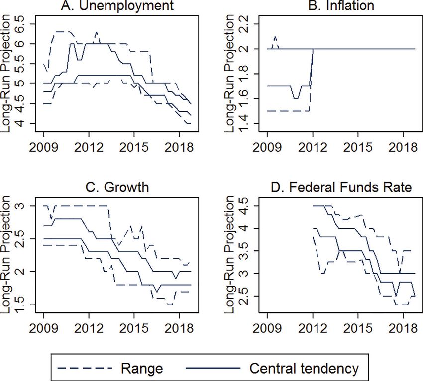
82         International Journal of Central Banking         June 2021

beliefs of consumers, professional forecasters, and central bankers
themselves (Mankiw, Reis, and Wolfers 2004; Boero, Smith, and
Wallis 2008; Romer and Romer 2008; Patton and Timmermann
2010; Coibion and Gorodnichenko 2012; Andrade and Le Bihan 2013;
Binder 2017c). Understanding the sources and nature of this dis-
agreement could have important implications for monetary policy
and central bank communication (Coibion and Gorodnichenko 2015;
Detmers 2016; Falck, Hoffmann, and Hurtgen 2017).
    Patton and Timmermann (2010) argue that disagreement in
shorter-horizon expectations mostly reflects differences in private
information, while disagreement about longer horizons reflects dif-
ferences in models. Andrade et al. (2016) show that forecasters in
the Blue Chip Financial Forecasts survey disagree even in very long-
horizon forecasts for output, inflation, and the federal funds rate,
and that this disagreement is time varying. They refer to this long-
horizon disagreement as fundamental disagreement, as it reflects dif-
fering views about slow-moving, unobserved economic fundamentals
like potential output, the natural interest rate, and the inflation
target. These unobserved fundamentals can be difficult to estimate
precisely in real time (Orphanides and Williams 2002; Laubach
and Williams 2016; Borio, Disyatat, and Juselius 2017; Holston,
Laubach, and Williams 2017).
    In this paper, I use data from the Federal Reserve Bank of
Philadelphia Survey of Professional Forecasters (SPF) to study fore-
casters’ beliefs and disagreement about the economy in the long
run, and related implications for central bank communication. I
exploit survey questions that ask forecasters whether they use the
natural rate of unemployment (u∗ ) to make forecasts and, if so,
asks for their estimates of u∗ . These questions provide explicit and
previously underutilized information about forecasters’ models and
beliefs.
    I show that forecasters’ responses to these questions are infor-
mative about their expectations-formation process. Forecasters who
say they use u∗ to forecast do appear to do so, in the sense that they
expect inflation to fall when they expect unemployment to be above
their own estimate of u∗ . The inflation expectations of forecasters
who report not using u∗ more closely resemble univariate forecasts
and are less sensitive to the unemployment gap or output gap.
These results are a novel contribution to the literature on the model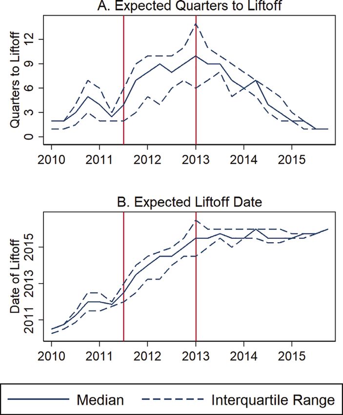
Vol. 17 No. 2       Central Bank Communication and Disagreement                 83

consistency of survey forecasts (Pierdzioch, Rulke, and Stadtmann
2011; Rulke 2012; Drager, Lamla, and Pfajfar 2016).1
    These results also provide empirical support for the general
premise of heterogeneous agent models with two types of private
agents, distinguished by their expectations formation (Andrade et al.
2018; Beqiraj, Di Bartolomeo, and Di Pietro 2019). In several papers,
the two types are “credibility believers” (also called “fundamental-
ists”), who trust the central bank, expect future inflation to be near
the central bank’s inflation target, and use a Phillips curve, and
“adaptive expectations users” (also called “naive” agents), who use
only past inflation to forecast future inflation (Busetti et al. 2017;
Goy, Hommes, and Mavromatis 2018; Cornea-Madeira, Hommes,
and Massaro 2019; Hommes and Lustenhouwer 2019). Having shown
that reported u∗ users appear to use a Phillips curve, I next show
that they resemble credibility believers in other ways as well. Most
notably, their long-run inflation expectations are closer to the Fed-
eral Reserve’s inflation target and more strongly anchored. Their
forecasts are also somewhat more accurate. Thus, while reported
use of u∗ cannot account for all differences between forecasters, it
does seem to provide a useful way to roughly categorize them into
these two types.
    The presence of credibility believers and adaptive expectations
users can have important implications for macroeconomic dynam-
ics and policy. Goy, Hommes, and Mavromatis (2018) study for-
ward guidance at the ZLB in a New Keynesian model with these
two types, assuming that only the credibility believers respond to
forward guidance.2 With a smaller share of credibility believers,

   1
     Pierdzioch, Rulke, and Stadtmann (2011) find that professional forecasters in
the G-7 make forecasts consistent with Okun’s law. Rulke (2012) finds that fore-
casters in Asian-Pacific countries use Okun’s law and the Phillips curve. Drager,
Lamla, and Pfajfar (2016) show that the share of U.S. consumers and forecast-
ers holding expectations consistent with the Fisher equation, Taylor rule, and
Phillips curve is time varying and that central bank communication can facilitate
understanding of these rules.
   2
     As in Campbell et al. (2012), forward guidance may be Delphic or Odyssean.
Delphic forward guidance conveys information about the central bank’s outlook,
while Odyssean forward guidance is interpreted as a commitment to deviate from
the central bank’s policy rule in the future, keeping rates “lower for longer” when
inflation and growth later rise (Eggertsson and Woodford 2003; Campbell et al.
2019).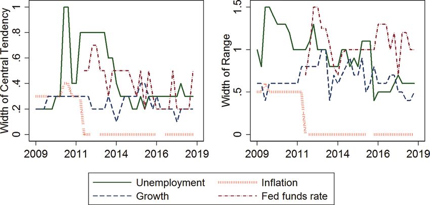
84           International Journal of Central Banking                 June 2021

forward guidance is less effective. Thus, the presence of adaptive
expectations users helps resolve the “forward-guidance puzzle,” or
the implausibly large responses of macroeconomic variables to for-
ward guidance in standard New Keynesian models with rational
expectations (Del Negro, Giannoni, and Patterson 2013; McKay,
Nakamura, and Steinsson 2016).3 To test whether the forecast-
ers who report using u∗ resemble credibility believers with respect
to forward guidance, I focus on the threshold-based forward guid-
ance issued in December 2012. I find that, indeed, forecasters who
report using u∗ were less likely to expect liftoff with unemployment
above the 6.5 percent threshold announced in the FOMC’s forward
guidance.
    Monetary policymakers communicate not only about the future
path of the policy rate but also about their projections of future
conditions and estimates of important parameters, including u∗ . The
quarterly Summary of Economic Projections (SEP) publishes indi-
vidual FOMC participants’4 anonymized projections for real gross
domestic product (GDP) growth, the unemployment rate, and infla-
tion at several horizons. Longer-run projections for growth, unem-
ployment, and headline inflation were added to the SEP in Febru-
ary 2009, and projections of the longer-run federal funds rate were
added in January 2012.5 The longer-run inflation projections were
widely interpreted as an informal inflation target until the January
2012 “Statement on Longer-Run Goals and Monetary Policy Strat-
egy” made the 2 percent inflation target explicit (Orphanides 2019).
According to Bernanke (2016b), the longer-run unemployment, out-
put growth, and federal funds rate projections can be interpreted

   3
     Other papers that introduce departures from rational expectations, including
imperfect knowledge and learning, to attempt to resolve the forward-guidance
puzzle include Ferrero and Secchi (2010), Cole (2015), Honkapohja and Mitra
(2015), and Eusepi and Preston (2018).
   4
     Following Bernanke (2016a), I use “FOMC participants” to refer to the seven
Board governors and 12 Reserve Bank presidents who contribute projections to
the SEP. “FOMC members” refers to a subset of participants, the seven Board
members, the president of the Federal Reserve Bank of New York, and a rotating
group of 4 of the remaining 11 Reserve Bank presidents.
   5
     https://www.federalreserve.gov/monetarypolicy/timeline-summary-of-
economic-projections.htm.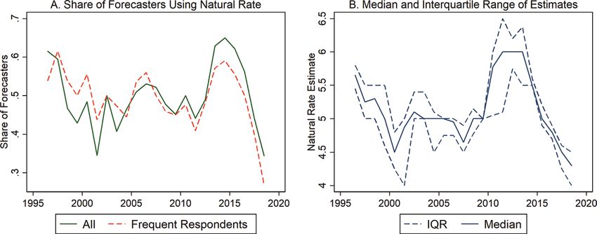
Vol. 17 No. 2      Central Bank Communication and Disagreement               85

as estimates of u∗ , potential output growth (y ∗ ), and the “neutral”
federal funds rate (r∗ ).6
    Faust (2016) characterizes the SEP as decentralized communica-
tion, as it reveals the diversity of policymakers’ views without clari-
fying how this diversity will affect committee policy choices. In con-
trast, centralized communication, like the threshold-based forward
guidance, clarifies how the FOMC intends to react to incoming infor-
mation. Faust argues that decentralized communication can poten-
tially lead to cacophony and confusion.7 For this reason, Bernanke
(2016a) judges that the SEP “remains a controversial part of the
Fed’s communications toolkit, and it has sometimes confused more
than enlightened” (also see Thornton 2015, Olson and Wessel 2016,
and Bundick and Herriford 2017).
    Decentralized communications do not fit neatly into the forward-
guidance model of Goy, Hommes, and Mavromatis (2018), who
assume that the central bank communicates with perfect precision,
though they note that this assumption is not always realistic. The
final section of this paper focuses on the FOMC’s longer-run unem-
ployment projections, documenting how and when the FOMC par-
ticipants have disagreed with each other and with the private sec-
tor, discussing possible sources of disagreement and implications for
credibility.
    This paper contributes to several other strands of literature,
including strands that use survey measures of expectations to study
inflation targeting and expectations anchoring (Davis 2012; Kumar
et al. 2015; Binder 2017a), to measure the effects of unconven-
tional monetary policy on private-sector expectations (Bauer and
Rudebusch 2013; Swanson and Williams 2014; Engen, Laubach, and
Reifschneider 2015; Andrade et al. 2018), or to analyze the nature
of information rigidities and the expectations-formation process
(Mankiw, Reis, and Wolfers 2004; Coibion and Gorodnichenko
2012). The paper also contributes to a literature on why mone-
tary policymakers disagree and how they communicate disagree-
ment. Nechio and Regan (2016) show that monetary policymakers’

   6
     FOMC participants also communicate about these estimates in speeches; e.g.,
see Clarida (2019).
   7
     Papers that suggest that more transparency is not always optimal include
Morris and Shin (2002), Thornton (2003), Stasavage (2007), and Sunstein (2017).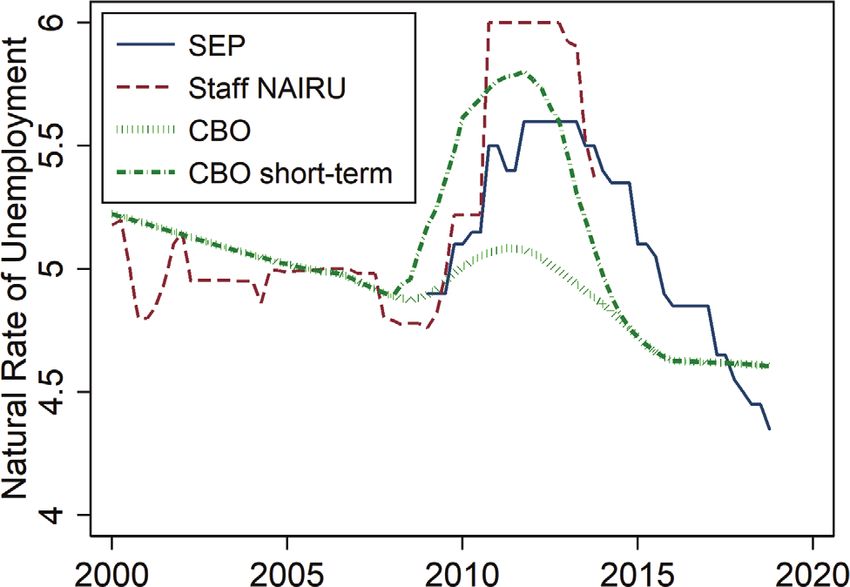
86          International Journal of Central Banking          June 2021

speeches reveal a diverse set of views among the FOMC. Hayo and
Neuenkirch (2013) and Jung and Latsos (2015) show that regional
economic variables affect the interest rate preferences and commu-
nications of Federal Reserve presidents.
    Finally, the paper contributes to the literature on the natural rate
hypothesis (NRH) and its use by policymakers. Friedman (1968)
famously argued that there is no long-run tradeoff between infla-
tion and unemployment; rather, unemployment returns to its “nat-
ural” rate in the long run. This natural rate is the rate that would
be observed when prices and wages have had time to fully adjust
to balance supply and demand, and depends on structural factors
characterizing the labor market (Walsh 1998).
    Blanchard (2018) reviews the arguments and empirical evidence
for and against two subhypotheses of the NRH: the independence
subhypothesis—that there exists a natural rate of unemployment
independent of monetary policy—and the accelerationist subhypoth-
esis—that monetary policy cannot sustain unemployment below u∗
without higher and higher inflation. First, there is some evidence of
hysteresis, or path dependence in the natural rate of unemployment,
which challenges the independence hypothesis (Ball 2009; Abraham
et al. 2019; Yagan 2019). Second, prolonged high unemployment
after 2009 did not lead to lower and lower inflation, which challenges
the accelerationist hypothesis, though alternative explanations for
the “missing disinflation” have been suggested (Coibion and Gorod-
nichenko 2015). Farmer (2013) also critiques the usefulness of the
NRH in explaining inflation dynamics.
    Several authors estimate policymakers’ beliefs about u∗ statis-
tically, via estimation of a model of the economy and of policy-
makers’ learning dynamics (Orphanides and Williams 2005, 2006;
Sargent, Williams, and Zha 2006; Williams 2006). Typically, these
models include an IS curve and a Phillips curve, written in terms
of time-varying natural rates of unemployment and interest that
are unobservable to policymakers but follow some specified data-
generating process, and a policymaker loss function. Policymakers’
misperceptions of u∗ can have important implications for inflation
dynamics and may have contributed to the Great Inflation of the
1970s (DeLong 1997; Romer and Romer 2002; Reis 2003; Prim-
iceri 2006; Ashley, Tsang, and Verbrugge 2018). Orphanides and
Williams (2002) study a variety of generalized Taylor (1993)-type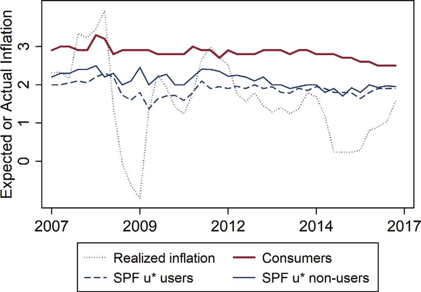
Vol. 17 No. 2   Central Bank Communication and Disagreement      87

monetary policy rules and show that the most robust rules under
such misperceptions are “difference rules” in which the policy rate
is raised or lowered from its previous level in response to infla-
tion and changes in economic activity. In contrast to these papers,
I use survey-based rather than model-derived measures of policy-
makers’ beliefs, and examine empirically the heterogeneity in both
policymaker and private-sector beliefs.
    Others use a narrative approach to study policymakers’ beliefs
about u∗ and the Phillips curve. For example, Romer and Romer
(2004) examine the narrative record to show that Federal Reserve
chairs since 1936 have held a variety of views about the sensitivity
of inflation to labor market slack and the level of u∗ . Meade and
Thornton (2012) use FOMC transcripts to evaluate the role of the
Phillips-curve framework in U.S. monetary policy from 1979 to 2003.
Most policymakers thought that inflation should be related to the
gap between aggregate demand and aggregate supply, but disagreed
about the usefulness of various gap measures in predicting inflation
and guiding policy. I similarly use a narrative approach to supple-
ment my analysis of policymakers’ beliefs. In addition to FOMC
transcripts and materials, I also examine the financial and popular
press, as my interest is in not only policymakers’ beliefs but also
private-sector beliefs.

2.   Forecasters’ Use of u∗ and Expectations Formation

The Federal Reserve Bank of Philadelphia Survey of Professional
Forecasters is a quarterly unbalanced panel of approximately 60
anonymous respondents. I make use of SPF forecasts for the civil-
ian unemployment rate (u), headline PCE inflation (π), and nom-
inal interest rates (i) at multiple horizons. Let xτj,t denote fore-
caster j’s expectation in quarter t of variable x at time τ , where
τ may be a calendar year or a quarter depending on context. SPF
respondents provide forecasts for the previous quarter (“backcast”),
current quarter (“nowcast”), and one, two, three, and four quar-
ters ahead, as well as annual average forecasts for the calendar
year in which the survey is conducted and the following calen-
dar year. Beginning in 2009:Q2 and 2009:Q3, respectively, fore-
casters also provide unemployment and three-month Treasury-bill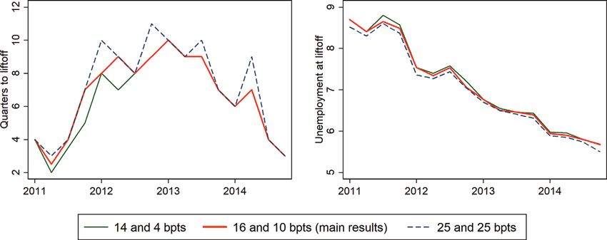
88         International Journal of Central Banking         June 2021

(T-bill) rate forecasts for the subsequent two calendar years. Since
2007:Q1, the SPF collects forecasts of personal consumption expen-
ditures (PCE) inflation for an additional calendar year and aver-
aged over the next five years (from the fourth quarter in the year
before the survey year to the fourth quarter of the year that is
five years beyond the survey year). SPF T-bill forecasts are for
the quarterly or annual average of the underlying daily levels and
unemployment forecasts for the average of the underlying monthly
levels. Quarterly PCE forecasts refer to annualized quarter-over-
quarter percent changes of the quarterly average seasonally adjusted
price index, and annual PCE forecasts refer to inflation from the
fourth quarter of the previous year to the fourth quarter of the year
indicated.
    A special SPF segment in 2009 asks respondents about their fore-
casting methods. Of the 25 forecasters who answered this optional
segment, 20 say they use a model with subjective adjustments, 1
uses a model alone, and 4 use just experience and intuition. Of those
using a model, 6 say they use a structural model, 3 use univariate or
multivariate time-series forecasting, and 11 use some combination.
Respondents to the special segment are not identified by forecaster
ID, so their reported forecasting methods cannot be matched with
their responses to other questions. However, another question on the
survey provides information about forecasters’ models and methods
that can be matched with their forecasts. Namely, in the third quar-
ter of each year since 1996, the SPF asks whether respondents use
the natural rate of unemployment (u∗ ) in forecasting and, if so, asks
for their estimate of u∗ .
    Panel A of figure 1 shows the share of forecasters who report
using u∗ to forecast over time. The share was around 50 percent
during the ZLB period, peaked at 65 percent in 2014, then declined
to 34 percent in 2018. While 124 forecasters have responded at least
once to the question of whether they use u∗ , some of these fore-
casters have only responded a few times. To address concerns about
compositional effects, I also consider the sample of 30 forecasters
who have responded to this question in at least 10 years. The share
using the natural rate is similar for the full sample and frequent
responders.
    Panel B shows how the median and interquartile range of esti-
mates of u∗ have evolved over time. In 2009:Q3, the 25th and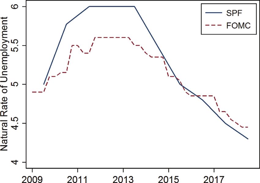
Vol. 17 No. 2      Central Bank Communication and Disagreement             89

Figure 1. SPF Forecasters’ Use and Estimates of Natural
                Rate of Unemployment

Notes: Data are from SPF. Frequent respondents are those that provide at least
10 responses to the question of whether they use the natural rate of unemploy-
ment.

75th percentile SPF forecasters agreed that u∗ was 5 percent. Two
years later, the median rose to 6 percent, and disagreement also
increased: the 25th percentile was 5.1 percent and the 75th percentile
6.5 percent. The median remained at 6 percent in 2012 and 2013, and
fell to a record low of 4.3 percent in 2018:Q3. These estimates are
also similar for the frequent responders. Thus, forecasters disagree
about whether u∗ is a useful forecasting concept, and among those
forecasters who do use u∗ , there is also time-varying fundamental
disagreement about the level of u∗ .

2.1   Short-Run Inflation Expectations
What does it mean if a forecaster reports using the natural rate
of unemployment to forecast? Recall that according to Blanchard
(2018), a key implication of the NRH—typically embedded in a
Phillips curve—is that unemployment below u∗ will lead to higher
inflation. I test whether this implication is observed in forecasters’
inflation expectations.
   As a baseline, I consider the Phillips curve specification that
Williams (2006) uses to study policymakers’ beliefs about u∗ , which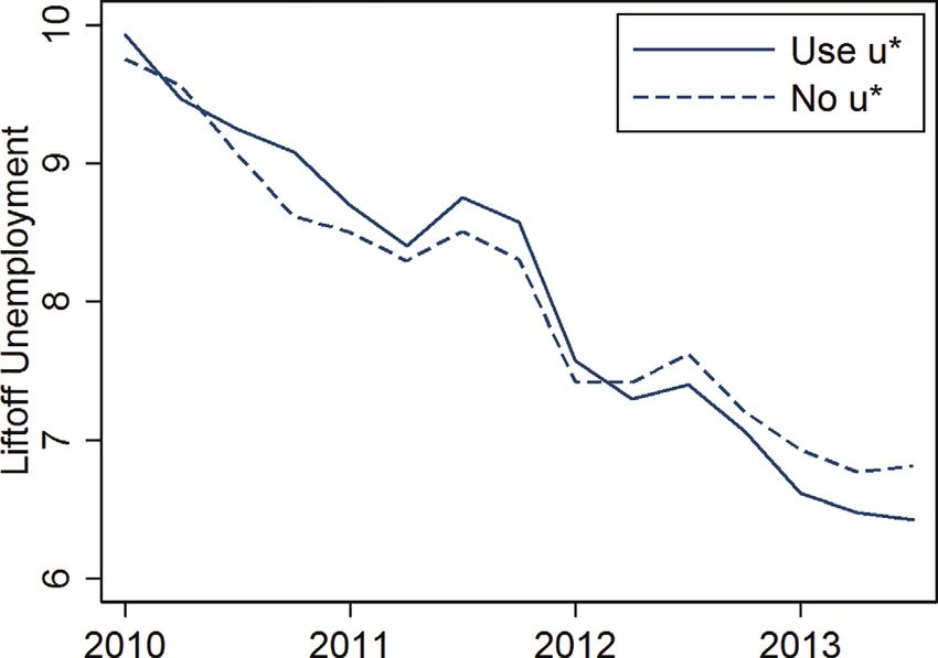
90            International Journal of Central Banking                 June 2021

relates inflation (π) to its own lags and the lagged unemployment
gap:8

             πt = γ1 πt−1 + γ2 πt−2 + γ3 (ut−1 − u∗t−1 ) + νt .                (1)

    For forecasters who provide an estimate u∗j,t , I can iterate equa-
tion (1) forward one period, apply the expectations operator with
respect to forecaster j in quarter t, and estimate the coefficients
                                                                   t+1
by regressing her one-quarter-ahead forecast of inflation (πj,t         ) on
                                             t        t−1
her nowcast and backcast of inflation (πj,t and πj,t ) and her per-
ception of the unemployment gap (utj,t − u∗j,t ).9 The first column of
table 1 shows that the estimate of γ3 is negative (−0.14) and sta-
tistically significant, as expected. Moreover, it is within the range
of estimates that Williams (2006) obtains from rolling regressions
using realized data from 1950 to 2003. The median of his rolling
regression estimates is −0.23.
    In the second column, I include the unemployment gap using the
forecaster’s own estimate u∗j,t as well as using the Congressional Bud-
get Office (CBO) estimate u∗CBO,t . Only the coefficient on utj,t −u∗j,t is
negative and statistically significant (though of course utj,t − u∗CBO,t
and utj,t − u∗j,t are highly correlated). Thus forecasters do appear to
use the estimate of u∗ that they personally report.
    In columns 3 and 4 I compare the expectations formation of fore-
casters who claim to use the natural rate with those who claim not
to. Since the latter do not provide estimates of u∗ , I use utj,t −u∗CBO,t
as the measure of the unemployment gap in both columns for the
sake of comparability. The coefficient on the unemployment gap
is less than half the magnitude of that for the forecasters who

   8
     Williams (2006) includes several additional lags of inflation and imposes a
unity sum on the coefficients; for simplicity I just include two lags with no con-
straint on the coefficients. Williams’s model is a version of the Rudebusch and
Svensson (1999) model, but written with a time-varying u∗ instead of output
gap.
   9
     Note that by using nowcasts and backcasts of inflation to estimate equation
(1), I avoid the need to make assumptions about forecasters’ real-time infor-
mation about macroeconomic variables, but instead rely on their self-reported
knowledge of conditions at time t and t − 1. This is useful because inflation data
are revised frequently, so analysis that assumes that ex post revised data are part
of agents’ information sets can be misleading (Orphanides 2001).
Table 1. The Natural Rate Hypothesis and SPF Inflation Expectations
(1) (2) (3) (4) (5) (6) (7) (8) (9)
π t+1 π t+1 π t+1 π t+1 π t+1 π t+1 π t+1 π t+1 π t+1
Vol. 17 No. 2
j,t j,t j,t j,t j,t j,t j,t j,t j,t
t
πj,t 0.28∗∗∗ 0.26∗∗∗ 0.26∗∗∗ 0.33∗∗∗ 0.24∗∗∗ 0.32∗∗∗
(0.03) (0.03) (0.03) (0.04) (0.02) (0.04)
t−1
πj,t −0.00 −0.01 −0.02 −0.03 −0.02 −0.03
(0.03) (0.03) (0.03) (0.02) (0.03) (0.02)
t+4
πj,t 0.25∗∗ 0.25∗∗ 0.47∗∗∗
(0.11) (0.12) (0.15)
utj,t − u∗j,t −0.14∗∗∗ −0.22∗∗∗ −0.15∗∗∗
(0.02) (0.06) (0.03)
utj,t − u∗CBO,t 0.06 −0.13∗∗∗ −0.05∗∗∗ −0.13∗∗∗ −0.07∗∗∗
(0.06) (0.02) (0.01) (0.02) (0.01)
Output Gap 0.13∗∗∗ 0.04∗∗
(0.02) (0.02)
Constant 1.43∗∗∗ 1.48∗∗∗ 1.52∗∗∗ 1.49∗∗∗ 1.57∗∗∗ 1.51∗∗∗ 1.39∗∗∗ 1.41∗∗∗ 1.11∗∗∗
(0.07) (0.08) (0.08) (0.09) (0.06) (0.10) (0.18) (0.21) (0.35)
N 827 720 720 679 847 696 822 838 673
2
Rw 0.28 0.25 0.25 0.30 0.26 0.30 0.08 0.10 0.09
Rb2 0.47 0.43 0.43 0.45 0.32 0.46 0.35 0.31 0.46
Sample Use u∗ Use u∗ Use u∗ No u∗ Use u∗ No u∗
Notes: Standard errors are in parentheses. ***, **, and * denote p < 0.01, p < 0.05, and p < 0.10, respectively. Time sample is
2007:Q1 through 2018:Q3. Data are from the Survey of Professional Forecasters (SPF). Dependent variable is forecast for next-quarter
Central Bank Communication and Disagreement
PCE inflation. u∗i,t is the respondent’s estimate of natural rate and u∗CBO,t is the CBO estimate. In columns 4 and 6, sample is the
respondents who report that they do not use u∗ .
9192 International Journal of Central Banking June 2021
use u∗ .10 Also note that the coefficient on inflation is 0.33, com-
pared with 0.26 for the u∗ users. Quarterly PCE inflation has an
AR(1) coefficient of 0.30 since 1996 and 0.36 after 2008.
It is possible that respondents who report not using u∗ do use
a Phillips curve to forecast, but with the output gap in place of
the unemployment gap. Columns 5 and 6 are analogous to 3 and
4, but with the output gap in place of the unemployment gap.11
The coefficient estimate on the output gap for the reported non-
users of u∗ users is again less than half of that for reported u∗
users. Results are robust to alternative specifications of the Phillips
curve in (1), including forward-looking specifications. For example,
the final three columns are analogous to columns 1, 3, and 4 but
t+4 t t−1
include πj,t as a regressor in place of πj,t and πj,t , and results are
similar.
In summary, forecasters who report using versus not using u∗
appear to be distinct in how they form short-run inflation expecta-
tions, and in particular in their beliefs about the Phillips curve.
The u∗ users seem to rely more on a Phillips curve to forecast
short-run inflation, much like the “credibility believers” in the
models of Goy, Hommes, and Mavromatis (2018), Cornea-Madeira,
Hommes, and Massaro (2019), and others.12 The non-users do not
perfectly resemble the “adaptive expectations” or “naive” agents, as
their inflation forecasts do rely somewhat on their unemployment
forecasts, but their inflation backcasts do explain a much larger
share of the variance in their inflation forecasts,13 so their beliefs
can be more reasonably approximated as following a univariate
model.
10
This difference is statistically significant. If I instead run the regression with
both groups of forecasters, and interact the unemployment gap with a dummy
variable indicating that the forecaster uses u∗ , the coefficient on the interaction
term is negative and statistically significant.
∗
11
The output gap is defined as 100 y−y y∗
, where y ∗ is the CBO estimate of
potential real GDP (Federal Reserve Economic Data (FRED) series GDPPOT)
and y is real GDP (FRED series RGDPC1).
12
In these models, the Phillips curve is specified in terms of marginal cost; since
SPF respondents do not provide marginal cost forecasts, I instead use the output
or unemployment gap.
13 t+1 t−1
Regression of πj,t on πj,t has an R2 value about three times higher for
non-users than for users.Vol. 17 No. 2 Central Bank Communication and Disagreement 93
2.2 Long-Run Inflation Expectations
Another important feature of the credibility believers in the models
of Cornea-Madeira, Hommes, and Massaro (2019) and others is that
they expect future long-run inflation to be equal to the inflation
target of the central bank. Busetti et al. (2017) and Hommes and
Lustenhouwer (2019) use models with credibility believers and naive
agents specifically to study inflation targeting.
January 2012 marked the first explicit announcement of a quan-
titative inflation target by the Fed, though the Fed had been
influenced by the inflation-targeting framework long before this
announcement (Bernanke 2003; Thornton 2012). Forecasters who
use u∗ were more aware that the Fed had an informal inflation tar-
get before the 2012 announcement, possibly inferring this from the
longer-run inflation projections in the SEP. In a 2007:Q4 special
questionnaire, among SPF respondents who have reported at least
once that they use u∗ in forecasting, 57 percent believed that the Fed
had a numerical target for inflation, compared with just 30 percent
of other respondents.
Figure 2 plots the median five-year-ahead inflation expectations
of each group as well as the longer-run inflation expectations of
respondents to the Michigan Survey of Consumers and realized infla-
tion. On average, the u∗ -users’ long-run inflation expectations are
23 basis points lower than the non-users’ expectations, are closer to
the inflation target, and fell more in the Great Recession. Non-users’
expectations are closer to and more correlated with the consumers’
expectations: the correlation between non-users’ and consumers’
inflation expectations is 0.46, and between users’ and consumers’
expectations 0.23.
The communication of a numerical target for long-run inflation
is intended to make long-run expectations more anchored, or less
responsive to shocks. In particular, if expectations are well anchored,
long-run inflation expectations should be minimally responsive to
changes in shorter-run expectations (Bernanke 2007; Davis 2012).
In table 2, I regress forecasters’ revisions to five-year-ahead infla-
5y 5y 5y
tion forecasts (Δπj,t = πj,t − πj,t−1 ) on revisions to forecasts for
the current quarter (Δπj,tt t
= πj,t − πj,t−1
t
). The sample in the first
column is forecasters who report using the natural rate at least once
(N Rj = 1), and in the second column is forecasters who never report94 International Journal of Central Banking June 2021
Figure 2. Long-Run Inflation Expectations of Consumers
and Professional Forecasters by Use of u*
Notes: The figure shows median 5- to 10-year inflation expectations of Michigan
Survey of Consumers respondents and median 5-year PCE inflation expectations
of SPF forecasters who report using or not using the natural rate of unemploy-
ment to forecast. Realized inflation refers to the percent change in the PCE price
index from one year previous.
using the natural rate (N Rj = 0). The natural rate users revise their
long-run expectations up 3 basis points for each percentage-point
increase in their expectations of current-quarter inflation, compared
with 10 basis points for non-users. The R2 is also much higher for the
non-users. Column 3 uses the full sample of forecasters but includes
t
an interaction of Δπj,t and N Rj . The coefficient on the interaction
term is negative and statistically significant.
In the fourth column, I consider whether the expectations of the
natural rate users became more anchored relative to those of the
non-users after the announcement of the inflation target in 2012.
This is a diff-in-diff-in-diff specification with the interaction term
P ostt ∗N Rj ∗Δπj,t
t
, where P ostt denotes that t is after the announce-
ment. The coefficient on the three-way interaction term is negative
and statistically significant, suggesting that the announcement may
have been more effective at anchoring the expectations of forecasters
who use the natural rate.Vol. 17 No. 2 Central Bank Communication and Disagreement 95
Table 2. Belief in the Natural Rate Hypothesis and
Anchoring of Long-Run Inflation Expectations
(1) (2) (3) (4)
Δπ 5y
j,t Δπ 5y
j,t Δπ 5y
j,t Δπ 5y
j,t
t
Δπj,t 0.03∗∗∗ 0.10∗∗∗ 0.10∗∗∗ 0.07∗∗∗
(0.01) (0.02 (0.02) (0.02)
t
NR*Δπj,t −0.08∗∗∗ −0.05∗∗
(0.02) (0.02)
t
Post*NR*Δπj,t −0.11∗∗∗
(0.04)
Post*NR −0.00
(0.02)
t
Post*Δπj,t 0.12∗∗∗
(0.04)
N 1,005 204 1,209 1,209
R2 0.02 0.13 0.05 0.06
Sample Use u* No u* All All
Notes: Standard errors are in parentheses. ***, **, and * denote p < 0.01, p < 0.05,
and p < 0.10, respectively. Time sample is 2007:Q1 through 2018:Q3. Data are from
the SPF. Dependent variable is revision in forecast for five-year-ahead PCE infla-
tion. “Post” denotes that the survey date is after the January 2012 inflation target
announcement. “NR” denotes that the respondent has reported at least once that
she uses the natural rate of unemployment to forecast. Regressions include a constant
term and forecaster fixed effects.
2.3 Credibility of Forward Guidance
At the ZLB, central banks’ ability to influence private-sector expec-
tations is important; a central bank can conduct monetary easing
if it can generate expectations that it will keep the policy rate low
to allow above-target inflation and above-trend output in the future
(Krugman 1998; Eggertson 2006; Boneva, Harrison, and Waldron
2018). Forward guidance can thus be interpreted as communica-
tion about future deviations from the central bank’s policy rule
(Campbell et al. 2019).
In Goy, Hommes, and Mavromatis (2018), only the credibil-
ity believers respond to the central bank’s forward guidance. I
test whether the reported u∗ users resemble credibility believers in
this respect. I focus on the “threshold-based” forward guidance of96 International Journal of Central Banking June 2021
December 2012 which announced that an “exceptionally low range
for the federal funds rate will be appropriate at least as long as the
unemployment rate remains above 6-1/2 percent, inflation between
one and two years ahead is projected to be no more than a half per-
centage point above the Committee’s 2 percent longer-run goal, and
longer-term inflation expectations continue to be well anchored.”
This guidance was intended to be less ambiguous, and hence better
able to guide expectations, than the open-ended guidance issued in
December 2008 (Woodford 2012; Williams 2013a).
Swanson and Williams (2014) use multi-horizon forecast data
from Blue Chip to infer when private forecasters expected “liftoff”
from the ZLB. Before the start of calendar-based forward guidance,
the median Blue Chip forecaster expected liftoff in about four quar-
ters. Expected time to liftoff increased in the calendar-based guid-
ance period. Since the Blue Chip data has a maximum horizon of
six quarters, for part of the calendar-based forward-guidance period
they can only infer that the median forecaster expects liftoff in seven
or more quarters. I conduct a similar exercise using the SPF data.
Since the SPF data are available at longer horizons, I avoid the top-
coding issue and can observe not only the median but also nearly
the full distribution of expected liftoff dates. See the appendix for
details.
I also compute expected unemployment at expected liftoff for
each forecaster and survey date. If an SPF forecaster expects liftoff
within the next four quarters, I use her quarterly forecast for unem-
ployment in the corresponding quarter as an estimate of her expected
liftoff conditions. If she expects liftoff at a later date, I linearly inter-
polate between her annual average unemployment forecasts to con-
struct estimates of her expectations of unemployment at each quar-
terly horizon, and use the interpolated unemployment and inflation
forecasts corresponding to my estimate of her expected liftoff date.14
In 2013, among forecasters who did not report using u∗ , only
33 percent expected unemployment below 6.5 percent at liftoff,
compared with 70 percent of forecasters who did report using u∗ .
14
I focus on expected unemployment rather than expected inflation at expected
liftoff since the PCE inflation forecasts are available for one less calendar year than
the unemployment and T-bill forecasts, and since the 6.5 percent unemployment
threshold is clearer that the inflation-related thresholds.Vol. 17 No. 2 Central Bank Communication and Disagreement 97
Table 3. Mean Squared Forecast Errors by Use of u ∗
u 1Q u 4Q r 1Q r 4Q π 1Q π 4Q
Non-users of u∗ 0.15 1.11 0.30 2.17 3.64 3.79
Users of u∗ 0.11 0.84 0.22 1.85 4.09 3.61
p-value 0.001 0.01 0.02 0.06 0.50 0.79
Notes: Data are from the SPF. The table shows forecasters’ mean squared forecast
error by reported use of u∗ for unemployment, interest rate (T-bill), and PCE infla-
tion forecasts at the one-quarter and four-quarter horizons. The final row shows the
p-value for the test of statistically significant difference in mean between the non-
users and users of u∗ . Unemployment and interest rate forecast data are available
1996:Q3 to 2018:Q3; inflation forecast data are available 2007:Q1 through 2017:Q3.
Thus, this aspect of forward guidance was more credible among the
reported u∗ users.
2.4 Forecast Accuracy and Composition of Types
Dragar, Lamla, and Pfajfar (2016) show that “model-consistent”
forecasters—those who make forecasts consistent with the Fisher
equation, Taylor rule, and Phillips curve—tend to have greater fore-
cast accuracy. I check whether forecasters who report using u∗ like-
wise make more accurate forecasts. Table 3 reports the mean squared
forecast error for unemployment, nominal interest rate, and inflation
forecasts at the one-quarter-ahead and four-quarter-ahead horizons
by reported use of u∗ . The forecasters who report not using u∗ have
larger forecast errors, on average, for unemployment and interest
rates at both horizons. The difference in accuracy is statistically sig-
nificant for unemployment at both horizons and for interest rates at
the one-quarter horizon, and marginally significant (p-value = 0.06)
for interest rates at the four-quarter horizon. The average difference
in inflation forecast accuracy is not statistically significant.
The models with credibility believers and naive agents make
no assumptions about which type makes more accurate forecasts.
Rather they assume, as in Brock and Hommes (1997) and Branch
et al. (2004), that agents switch heuristics based on “relative fit-
ness,” or some history of relative forecasting performance.15 That
15
This assumption formalizes Simon’s (1984) suggestion that decisionmaking
can be modeled as a rational choice between a set of different heuristics.98 International Journal of Central Banking June 2021
is, if the forecasts made by credibility believers become relatively
less accurate than the adaptive expectations forecasts, then a larger
share of agents will use adaptive expectations.
In Cornea-Madeira, Hommes, and Massaro (2019), agents switch
between being credibility believers and adaptive expectations users
based strictly on the relative inflation-forecasting performance of the
two heuristics. Cornea-Madeira, Hommes, and Massaro estimate the
share of credibility believers over time using aggregate data (with-
out survey data on expectations) and a New Keynesian model. They
find that the average share of credibility believers has declined in
recent years, and posit that in the aftermath of the financial cri-
sis, prolonged below-target inflation has improved the relative fore-
cast accuracy of simple univariate (“naive”) forecasts, reducing the
share of credibility believers. (See Busetti et al. 2017 for a similar
discussion.)
Recall from panel A of figure 1 that the share of u∗ users has
also declined in recent years. The share of u∗ users, which has mean
0.5 and standard deviation 0.08, is not as volatile as the estimated
share of credibility believers in Cornea-Madeira, Hommes, and Mas-
saro (2019), which has mean 0.33 and standard deviation 0.27. Part
of the difference in mean and volatility may reflect the difference
in sample periods, as the sample in Cornea-Madeira, Hommes, and
Massaro (2019) starts in 1964 and mine starts in 1996. But it is
also possible that forecasters’ choice of model depends on more than
just inflation forecast accuracy. Forecasters may consider the accu-
racy of forecasts for multiple variables, or type may be “sticky”
due to switching costs (cognitive or otherwise). Forecasters may also
evaluate the relative ease of using different models. For example, if
u∗ becomes highly variable and difficult to precisely estimate, they
may switch away from using models that rely on u∗ .16 Forecasters
may also be influenced by central bank communications or media
narratives about how the economy works.
16
The absolute number of forecasters that switch from reportedly using to not
using the natural rate or vice versa is fairly small: since 1997, only 39 forecasters
have switched from not using to using, and only 34 have switched from using
to not using. Thus it is difficult to test statistically for possible predictors of
switching behavior.Vol. 17 No. 2 Central Bank Communication and Disagreement 99
3. Federal Reserve Communication and Disagreement
about u∗
The previous section showed that forecasters who report using versus
not using the natural rate of unemployment are distinct in how they
forecast short- and long-run inflation. The u∗ users seem to resemble
“credibility believers,” including with respect to forward guidance at
the ZLB. Thus the time-varying share of u∗ users may have impor-
tant implications for central bank credibility and expectations for-
mation. But recall from figure 1 that even among reported u∗ users,
estimates of u∗ and disagreement about u∗ are also time varying.
These variations are worth understanding for several reasons.
First, section 2.1 showed that forecasters use their own esti-
mates of u∗ to form inflation forecasts. The negative estimate of γ3
in equation (1) implies that, all else equal, forecasters with higher
estimates of u∗ should have higher expectations of future inflation.
Thus disagreement about u∗ contributes to disagreement in inflation
expectations. This is also true for longer-run inflation expectations.
Panel regressions of five-year-ahead inflation expectations on u∗j,t
with time fixed effects have a coefficient estimate of 0.23 on u∗j,t ,
which is statistically significant with p < 0.05.17
Second, the quarterly Summary of Economic Projections pub-
lishes FOMC participants’ estimates of u∗ . The SEP is a decentral-
ized form of Fed communication (Faust 2016). Substantial disagree-
ment about u∗ among SPF forecasters, or between SPF forecast-
ers and FOMC participants, despite publication of the SEP, might
point to weaknesses in Federal Reserve communication, and might be
related to the subsequent reduction in reported u∗ users. As I will
show, both types of disagreement were especially high from 2011
through 2013, when many SPF forecasters became more pessimistic
than many FOMC participants about u∗ . Third, and relatedly, recall
from section 2.3 that in 2013:Q3, 33 percent of u∗ non-users and 70
percent of u∗ users expected unemployment below 6.5 percent at
liftoff. Among forecasters with an estimate of u∗ less than 6 percent
(the highest FOMC projection) in that quarter, 83 percent expected
17
If the regression includes forecaster fixed effects, the coefficient is 0.19, which
is statistically significant with p < 0.01.100 International Journal of Central Banking June 2021
unemployment below 6.5 percent at liftoff. For those with an esti-
mate of u∗ at least 6 percent, only 50 percent expected unemploy-
ment below 6.5 percent at liftoff.18 Thus forecasters who were more
pessimistic about u∗ than most of the FOMC were less likely to have
expectations consistent with the threshold-based forward guidance.
3.1 FOMC Projections of Longer-Run Unemployment
In the SEP, the five Board members and 12 presidents provide pro-
jections for several macroeconomic variables for the current calendar
year and up to three subsequent years, as well as for the “long run.”
The projections are not unconditional expectations, but are condi-
tional on appropriate monetary policy. Responses are anonymized
and cannot be linked from one meeting to the next.
Panel A of figure 3 summarizes FOMC projections of longer-
run unemployment from the SEP, which are available since 2009.
In 2009, the FOMC projections in 2009 displayed minimal disagree-
ment, with the central tendency from 4.8 to 5 percent. The width
of the central tendency of the FOMC projections subsequently rose,
and the midpoint of the central tendency increased. Since projec-
tions are conditional on appropriate monetary policy, the increasing
width of the central tendency could reflect growing divergence in
assumptions about appropriate policy.
These patterns are similar to those for the SPF: panel B of
figure 1 shows that in 2009:Q3, the majority of SPF respondents
who reported using u∗ also estimated that u∗ was 5 percent. In fact,
for forecasters that said they used u∗ , 57 percent reported an esti-
mate of 5 percent, and all estimates were between 4 percent and 6
percent. The median estimate and the interquartile range (disagree-
ment) both rose the next year and remained elevated throughout
the ZLB period. But most FOMC projections increased by less than
most SPF estimates of u∗ . As figure 4 shows, by 2011 through 2013,
the SPF median was around 50 basis points higher than the FOMC
midpoint. In 2013:Q3, the central tendency of the FOMC long-run
unemployment projections was 5.2 to 5.8 percent, and 55 percent of
SPF estimates of u∗ were above 5.8 percent.
18
This difference is statistically significant at the 10 percent level.Vol. 17 No. 2 Central Bank Communication and Disagreement 101
Figure 3. FOMC Longer-Run Projections
Notes: Summary of Economic Projections data accessed from FRED. The cen-
tral tendency excludes the three lowest and three highest projections. Variable
codes: UNRATERLLR, UNRATECTLLR, UNRATECTHLR, PCECTPIRHLR,
PCECTPIRLLR, PCECTPICTLLR, PCECTPICTHLR, PCECTPIRHLR,
GDPC1RHLR, GDPC1RLLR, GDPC1CTLLR, GDPC1CTHLR, GDPC1RHLR,
FEDTARRHLR, FEDTARRLLR, FEDTARCTLLR, FEDTARCTHLR, and
FEDTARRHLR.
The other panels of figure 3 summarize FOMC longer-run pro-
jections of PCE inflation, growth, and the federal funds rate, while
figure 5 shows the width of the central tendency and the range for
each longer-run projection over time. Notice that there is no dis-
agreement about longer-run inflation since the 2012 announcement
of a 2 percent target. Disagreement about longer-run growth did
not increase with disagreement about longer-run unemployment, but
rather stayed nearly constant as the midpoint longer-run growth102 International Journal of Central Banking June 2021
Figure 4. SPF Estimates and FOMC Projections of
Natural Rate of Unemployment
Notes: The solid line is the median SPF estimate of u*. The dashed line is
the midpoint of the central tendency for the SEP longer-run unemployment
projection.
estimate gradually declined. The longer-run federal funds rate pro-
jections, published since 2012, show substantial disagreement about
the longer-run policy rate as the midpoint estimate has fallen, which
may reflect the documented low precision in estimates of the natural
interest rate (Laubach and Williams 2016).
3.2 Definitions of u∗
Why did FOMC and SPF estimates of u∗ , which were so similar
in 2009, subsequently diverge? One possibility is that forecasters
and FOMC participants use different definitions of “natural rate of
unemployment.” Bernanke (2016b) says that the longer-run unem-
ployment projections in the SEP “can be viewed as estimates of
the ‘natural’ rate of unemployment, the rate of unemployment that
can be sustained in the long run without generating inflationary or
deflationary pressures.” The SPF respondents are not provided with
a definition of “natural rate of unemployment.”Vol. 17 No. 2 Central Bank Communication and Disagreement 103 Figure 5. FOMC Disagreement in Longer-Run Projections Notes: Summary of Economic Projections data accessed from FRED. The cen- tral tendency excludes the three lowest and three highest projections. Variable codes: UNRATERLLR, UNRATECTLLR, UNRATECTHLR, PCECTPIRHLR, PCECTPIRLLR, PCECTPICTLLR, PCECTPICTHLR, PCECTPIRHLR, GDPC1RHLR, GDPC1RLLR, GDPC1CTLLR, GDPC1CTHLR, GDPC1RHLR, FEDTARRHLR, FEDTARRLLR, FEDTARCTLLR, FEDTARCTHLR, and FEDTARRHLR. The natural rate of unemployment is often treated as synony- mous with the NAIRU (non-accelerating inflation rate of unemploy- ment), though the two concepts are distinct and play different roles in monetary policy (Estrella and Mishkin 1999). The NAIRU is the unemployment rate consistent with steady inflation in the near term, and thus plays a more direct role in policy conduct because it helps with forecasting inflation and achieving an inflation target. How- ever, its high variability and difficulty to measure (Staiger, Stock, and Watson 1997; Tasci and Verbrugge 2014) can make the NAIRU problematic to use when explaining policy actions to the public. See Espinosa-Vega and Russell (1997) for a detailed history of economic thought surrounding the NAIRU and the natural rate hypothesis. Meanwhile the natural rate, which is slower moving, serves as the appropriate benchmark for unemployment stabilization objectives (Walsh 1998). The distinction between the natural rate and the NAIRU may have been minimal in 2009 but larger in the subsequent years.
104           International Journal of Central Banking                June 2021

      Figure 6. SEP, Greenbook, and CBO Estimates of
         Natural Rate of Unemployment or NAIRU

Notes: The solid line is the midpoint of the central tendency for the SEP longer-
run unemployment projection. The dashed line is the real-time NAIRU estimate
from the Board of Governors, accessed from the Federal Reserve Bank of Philadel-
phia Greenbook Data Sets. CBO estimates of u* are accessed from FRED (series
NROU and NROUST).

Indeed, until recently, the CBO published a single series they referred
to as the “natural rate of unemployment (NAIRU)” (implicitly treat-
ing the natural rate and NAIRU as synonyms). But in 2008, the
CBO began distinguishing between a “long-run natural rate” and a
“short-run natural rate.” The latter, which incorporates temporary
factors, is more akin to the NAIRU in that it is used to gauge labor
market slack in the CBO projections of inflation.
    Figure 6 displays both of these CBO series over time. In 2009,
the longer-term and shorter-term CBO estimates were 4.9 percent
and 5.2 percent, respectively. But the longer-term estimate remained
near 5 percent, while the shorter-term estimate peaked at 5.8 percent
in 2011:Q4. Figure 6 also plots the midpoint of the SEP longer-run
unemployment, which rose much more than the longer-term CBO
estimate but less than the shorter-term CBO estimate.
    The Federal Reserve Bank of Philadelphia Real-Time Data
Research Center provides the “NAIRU Estimates from the Board of
Vol. 17 No. 2 Central Bank Communication and Disagreement 105
Governors,” which contains the Federal Reserve staff’s real-time esti-
mates of the NAIRU from the Greenbooks.19 The data are released
with a lag of at least five years; as of August 2019, the NAIRU data
are available through December 2013. This NAIRU estimate is also
plotted on figure 6. The staff NAIRU estimates rose from 5.0 percent
in 2009:Q3 to 6.0 percent in 2010:Q4, and remained at 6.0 per-
cent (well above the SEP midpoint but similar to the SPF median)
through 2012:Q4. By 2013:Q3, both the staff NAIRU estimate and
the SEP longer-run unemployment midpoint were 5.5 percent. Thus,
the SEP longer-run unemployment projections appear to be similar
to the staff NAIRU estimates in normal times, but the NAIRU is
a shorter-run concept that may rise more than the natural rate of
unemployment in recessions.
It is possible that some SPF respondents report estimates of the
(short-run) NAIRU while others report the (long-run) natural rate
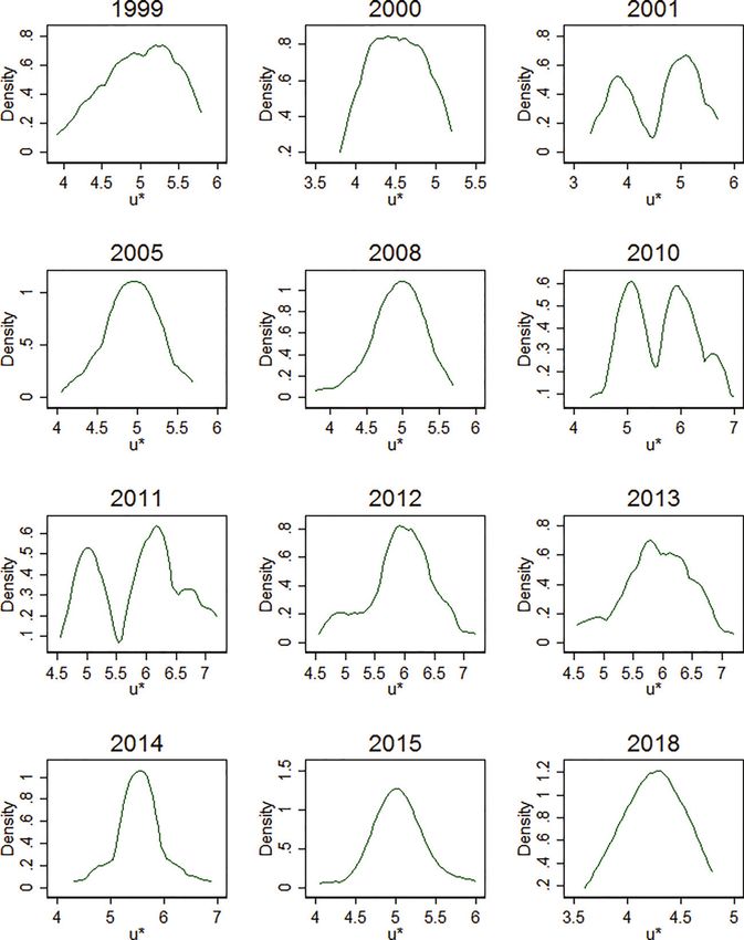
of unemployment. Figure 7 plots kernel density estimates of SPF
u∗ estimates in different years. The distribution of u∗ estimates is
unimodal in all years (including the years not displayed) except for
2001, 2010, and 2011, when it is clearly bimodal. In 2001, a recession
year with a sharp rise in unemployment, the modes are at 4 percent
and 5 percent, while in 2010 and 2011, the two modes are near 5 per-
cent and 6 percent, perhaps corresponding to a group of respondents
reporting the natural rate and another group reporting the NAIRU.
By 2012 and 2013, though the kernel density appears unimodal, the
popular responses are 5.5 percent, 6 percent, and 6.5 percent. The
lower estimates may still correspond to respondents reporting the
natural rate and higher estimates the NAIRU. This could explain
why disagreement among SPF forecasters and between the SPF and
the FOMC were both heightened in 2010 through 2013.
However, even among the FOMC participants, disagreement
about longer-run unemployment was especially high from 2010
through 2013. Moreover, as FOMC and SPF estimates of u∗ have
been repeatedly revised downward, the share of reported u∗ users
19
Data are available at https://www.philadelphiafed.org/surveys-and-data/
real-time-data-research. For comparative analysis of staff and FOMC members’
forecasts, see Romer and Romer (2008) and Binder and Wetzel (2018).106 International Journal of Central Banking June 2021
Figure 7. Kernel Density Estimates by Year of SPF
Estimates of u*
Notes: Data are from SPF. Kernel density estimates for forecasters’ estimate of
the natural rate of unemployment by year for select years. Epanechnikov kernel
with bandwidth 0.2.Vol. 17 No. 2 Central Bank Communication and Disagreement 107
has also fallen. The final subsection discusses other potential con-
tributors to disagreement and uncertainty about the natural rate
based on narrative evidence.
3.3 Narrative Evidence and Discussion
FOMC transcripts and speeches, media coverage, and the academic
literature provide some additional insights into the patterns that
appear in figures 1, 3, and 4. The rise in median or midpoint esti-
mates and disagreement about u∗ for both the SPF and the FOMC
corresponds to the timing of the “missing disinflation” puzzle. This
puzzle refers to the fact that inflation fell relatively little despite sus-
tained high unemployment in the aftermath of the Great Recession.
This missing disinflation led to uncertainty and disagreement about
whether the Phillips curve was “alive and well,” and about the extent
to which a rise in u∗ was the cause (Coibion and Gorodnichenko
2015).
Abraham (2015) notes that the idea that the labor market is
suffering from “skills mismatch” often becomes popular during pro-
longed periods of high unemployment. This does appear to be the
case following the Great Recession. Paul Krugman describes a con-
sensus by the news media that the high unemployment during and
after the Great Recession was structural, resulting from skills mis-
match.20 He argues that the media presented the skills mismatch
story as the known truth, despite weak evidence to support it. I
searched U.S. publications in the Nexis Uni database for the terms
“skill mismatch” or “skills mismatch” and “unemployment.” As
shown in figure 8, the volume of news coverage of skill mismatch
did indeed rise dramatically beginning in 2010 and peaking in 2012.
Reports of skill mismatch often accompanied discussions of the
unconventional policies introduced by the Fed at the ZLB, includ-
ing the quantitative easing (QE) programs (see Blinder 2010). Some
drew the conclusion that monetary policy, particularly QE3, would
have limited ability to reduce unemployment. For example, on
Bloomberg TV, John Ryding, Chief Economist and Founding Part-
ner at RDQ Economics, said, “Let’s remember that there’s certain
20
Paul Krugman, “Structural Unemployment: Yes, It Was Humbug,” New York
Times, August 4, 2017.You can also read