Cognitive Biases: Mistakes or Missing Stakes? 8168 2020 - ifo Institut
←
→
Page content transcription
If your browser does not render page correctly, please read the page content below
8168
                                                                      2020
                                                                      March 2020

Cognitive Biases: Mistakes or
Missing Stakes?
Benjamin Enke, Uri Gneezy, Brian Hall, David Martin, Vadim Nelidov,
Theo Offerman, Jeroen van de Ven
Impressum:

CESifo Working Papers
ISSN 2364-1428 (electronic version)
Publisher and distributor: Munich Society for the Promotion of Economic Research - CESifo
GmbH
The international platform of Ludwigs-Maximilians University’s Center for Economic Studies
and the ifo Institute
Poschingerstr. 5, 81679 Munich, Germany
Telephone +49 (0)89 2180-2740, Telefax +49 (0)89 2180-17845, email office@cesifo.de
Editor: Clemens Fuest
https://www.cesifo.org/en/wp
An electronic version of the paper may be downloaded
· from the SSRN website:       www.SSRN.com
· from the RePEc website:      www.RePEc.org
· from the CESifo website:     https://www.cesifo.org/en/wp
CESifo Working Paper No. 8168

      Cognitive Biases: Mistakes or Missing Stakes?
                                                 Abstract

Despite decades of research on heuristics and biases, empirical evidence on the effect of large
incentives – as present in relevant economic decisions – on cognitive biases is scant. This paper
tests the effect of incentives on four widely documented biases: base rate neglect, anchoring,
failure of contingent thinking, and intuitive reasoning in the Cognitive Reflection Test. In pre-
registered laboratory experiments with 1,236 college students in Nairobi, we implement three
incentive levels: no incentives, standard lab payments, and very high incentives that increase the
stakes by a factor of 100 to more than a monthly income. We find that cognitive effort as
measured by response times increases by 40% with very high stakes. Performance, on the other
hand, improves very mildly or not at all as incentives increase, with the largest improvements
due to a reduced reliance on intuitions. In none of the tasks are very high stakes sufficient to de-
bias participants, or come even close to doing so. These results contrast with expert predictions
that forecast larger performance improvements.
JEL-Codes: D010.
Keywords: cognitive biases, incentives.

                                           Benjamin Enke*
                                     Harvard University / MA / USA
                                        enke@fas.harvard.edu
                  Uri Gneezy                                               Brian Hall
            UC San Diego / CA / USA                            Harvard Business School / MA / USA
              ugneezy@ucsd.edu                                          bhall@hbs.edu
                 David Martin                                            Vadim Nelidov
         Harvard University / MA / USA                     University of Amsterdam / The Netherlands
               dmartin@hbs.edu                                          v.nelidov@uva.nl
                Theo Offerman                                           Jeroen van de Ven
  University of Amsterdam / The Netherlands                University of Amsterdam / The Netherlands
            T.J.S.Offerman@uva.nl                                      J.vandeVen@uva.nl
*corresponding author

March 6, 2020
The experiments in this paper were pre-registered on AsPredicted at https://aspredicted.org/blind.php?x=5jm93d
and received IRB approval from Harvard’s IRB. For excellent research assistance we are grateful to Tiffany Chang,
Davis Heniford, and Karim Sameh. We are also grateful to the staff at the Busara Center for Behavioral Economics
for dedicated support in implementing the experiments. We thank Thomas Graeber and Florian Zimmermann for
helpful comments.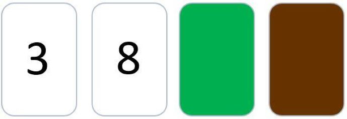
1    Introduction
Starting with Tversky and Kahneman (1974), the “heuristics and biases” program has
occupied psychologists and behavioral economists for nearly half a century. In a nutshell,
this voluminous and influential line of work has documented the existence and robust-
ness of a large number of systematic errors – “cognitive biases” – in decision-making.
    In studying these biases, psychologists often use hypothetical scenarios. Experimen-
tal economists criticize the lack of incentives, and use payments that amount to a couple
of hours of wages for the students participating in order to motivate them to put effort
into the task. Yet, non-experimental economists often raise concerns in response to find-
ings based on such incentives, arguing that people will exert more effort in high-powered
decisions, so that cognitive biases may be irrelevant for understanding real-world behav-
ior. In other words, just like experimental economists criticize psychologists for not in-
centivizing at all, non-experimental economists often criticize experimental economists
for using fairly small incentives. As Thaler (1986) states in his discussion of ways in
which economists dismiss experimental findings: “If the stakes are large enough, people
will get it right. This comment is usually offered as a rebuttal. . . but is also, of course, an
empirical question. Do people tend to make better decisions when the stakes are high?”
    We address this empirical question for two reasons. First, as noted by Thaler, a rele-
vant issue is to understand whether systematic departures from the rational economic
model are likely to appear only in the many small-stakes decisions that we make, or
also in decisions with high-powered incentives and large financial implications. Such
understanding can inform our modeling of important real-life decisions. Second, it is
of interest to understand the mechanisms behind cognitive biases. For example, a very
active recent theoretical and experimental literature attempts to identify the extent to
which different biases are generated by micro-foundations such as incorrect mental mod-
els, memory imperfections, or limited attention, where low effort often features as one
of the prime candidates.
    Perhaps somewhat surprisingly, systematic empirical evidence that looks at the effect
of very large incentives on cognitive biases is scant. The current paper targets this gap
in the literature. We conduct systematic tests of the effects of incentive size, and in par-
ticular the effects of very large incentives, on four well-documented biases. Our design
has three pay levels: no incentives, relatively small incentives that amount to standard
laboratory pay, and very high incentives that are 100 times larger than the standard
stake size and equivalent to more than one month’s income for our participants.
    We apply these stake-size variations to the following well-established biases: base
rate neglect (BRN); anchoring; failure of contingent thinking in the Wason selection
task; and intuitive reasoning in the Cognitive Reflection Test (CRT). Our interest in this

                                               1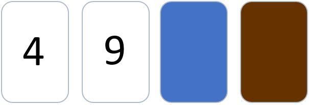
paper is not so much in these biases per se, but rather in the effects of varying the stake
size. We therefore selected these particular biases subject to the following criteria: (i)
the tasks that underlie these biases have an objectively correct answer; (ii) the biases
are cognitive in nature, rather than preference-based; (iii) standard experimental in-
structions to measure these biases are short and simple, which helps rule out confusion
resulting from complex instructions; and (iv) these biases all have received much atten-
tion and ample experimental scrutiny in the literature.¹ An added benefit of including
the CRT in our set of tasks is that it allows us to gauge the role of intuitions in generat-
ing cognitive biases: if it were true that higher stakes and effort reduced biases in the
CRT but not otherwise, then other biases are less likely to be primarily generated by
intuitions and a lack of deliberative thinking.
    Because there is a discussion in the literature about the frequency of cognitive biases
in abstractly vs. intuitively framed problems, we implement two cognitive tasks (base
rate neglect and the Wason selection task aimed at studying contingent thinking) in both
a relatively abstract and a relatively intuitive frame. Entirely abstract frames present only
the elements of a problem that are necessary to solve it, without further context. More
intuitive frames present a problem with a context intended to help people to relate it
to their daily life experiences. In total, we implement our three incentive conditions
with six types of tasks: abstract base rate neglect, intuitive base rate neglect, anchoring,
abstract Wason selection task, intuitive Wason selection task, and the CRT.
    We run our pre-registered experiments with a total of N = 1, 236 college students in
the Busara Center for Behavioral Economics in Nairobi, Kenya. We selected this lab to
run our experiments because of the lab’s ability to recruit a large number of analytically
capable students for whom our large-stakes treatment is equal to more than a month’s
worth of income. Participants are recruited among students of the University of Nairobi,
the largest and most prestigious public university in Kenya. While this sample is different
from the types of samples that are typically studied in laboratory experiments, the CRT
scores of these students suggest that their reasoning skills are similar to those of partici-
pants in web-based studies in the U.S., and higher than in test-taker pools at typical U.S.
institutions such as Michigan State, U Michigan Dearborn, or Toledo University.
    In the two financially incentivized conditions, the maximum bonus is 130 KSh ($1.30)

    ¹Base rate neglect is one of the most prominent and widely studied biases in belief updating (Grether,
1980, 1992; Camerer, 1987; Benjamin, 2019). Anchoring has likewise received much attention, with
widely cited papers such as Ariely et al. (2003); Epley and Gilovich (2006); Chapman and Johnson (2002).
Failure in contingent reasoning is a very active subject of study in the current literature, as it appears to
manifest in different errors in statistical reasoning (Esponda and Vespa, 2014, 2016; Enke, 2017; Enke and
Zimmermann, 2019; Martínez-Marquina et al., 2019). Finally, intuitive reasoning in the CRT is probably
the most widely implemented cognitive test in the behavioral sciences, at least partly because it is strongly
correlated with many behavioral anomalies from the heuristics and biases program (Frederick, 2005;
Hoppe and Kusterer, 2011; Toplak et al., 2011; Oechssler et al., 2009).

                                                     2
and 13,000 KSh ($130). Median monthly income and consumption in our sample are
in the range of 10,000–12,000 KSh, so that the high stakes condition offers a bonus of
more than 100% of monthly income and consumption. As a second point of compari-
son, note that our standard and high incentive levels correspond to about $23.50 and
$2,350 at purchasing power parity in the United States. We chose experimental pro-
cedures that make these incentive payments both salient and credible. We deliberately
selected the Busara lab for implementation of our experiments because the lab follows a
strict no-deception rule. In addition, both the written and the oral instructions highlight
that all information that is provided in the experimental instructions is true and that all
consequences of subjects’ actions will happen as described. Finally, the computer screen
that immediately precedes the main decision tasks reminds subjects of the possibility of
earning a given bonus size.
Because the focus of our paper is the comparison between high stakes and stan-
dard stakes, we implement only two treatment conditions to maximize statistical power
within a given budget. At the same time, to additionally gather meaningful information
on participants’ behavior without any financial incentives, the experiment consists of
two parts. In the first part, each subject completes the questions for a randomly selected
bias without any incentives. Then, the possibility of earning a bonus in the second part
is mentioned, and subjects are randomized into high or standard incentives for a cog-
nitive bias that is different from the one in the first part. Thus, treatment assignment
between standard and high stakes is random, yet we still have a meaningful benchmark
for behavior without incentives.
We find that, across all of our six tasks, response times – our pre-registered proxy for
cognitive effort – are virtually identical with no incentives and standard lab incentives.
On the other hand, response times increase by about 40% in the very high incentive
condition, and this increase is similar across all tasks. Thus, there appears to be a signif-
icant and quantitatively meaningful effect of incentives on cognitive effort that could in
principle translate into substantial reductions in the frequency of observed biases.
There are two ex ante plausible hypotheses about the effect of financial incentives
on biases. The first is that cognitive biases are largely driven by low motivation, so that
large stake size increases should go a long way towards debiasing people. An alternative
hypothesis is that cognitive biases reflect the high difficulty of rational reasoning and /
or high cognitive effort costs, so that even very large incentives will not dramatically
improve performance.
Looking at the frequency of biases across incentive levels, our headline result is that
cognitive biases are largely, and almost always entirely, unresponsive to stakes. In five
out of our six tasks, the frequency of errors is statistically indistinguishable between
standard and very large incentives, and in five tasks it is statistically indistinguishable
3between standard and no incentives. Given our large sample size, these “null results”
are relatively precisely estimated: across the different tasks, we can statistically rule out
performance increases of more than 3–18 percentage points. In none of the tasks did
cognitive biases disappear, and even with very large incentives the error rates range
between 40% and 90%.
The only task in which very large incentives produce statistically significant perfor-
mance improvements is the CRT. We also find some mildly suggestive evidence that
stakes matter more in the intuitive versions of base rate neglect and the Wason task.
A plausible interpretation of these patterns is that increased incentives reduce reliance
on intuitions, yet some problems are sufficiently complex for people that the binding
constraint is not low effort and reliance on intuitions but instead a lack of conceptual
problem solving skills. Our correlational follow-up analyses are in line with such an inter-
pretation: the within-treatment correlations between cognitive effort and performance
are always very small, suggesting that it is not only effort per se but at least partially
“the right way of looking at a problem” that matters for cognitive biases.
Our results contrast with the predictions of a sample of 68 experts, drawn from
professional experimental economists and Harvard students with exposure to graduate-
level experimental economics. These experts predict that performance will improve by
an average of 25% going from no incentives to standard incentives, and by another 25%
going from standard to very high incentives. While there is some variation in projected
performance increases across tasks, these predictions are always more bullish about the
effect of incentives than our experimental data warrant.
Our paper ties into the large lab experimental literature that has investigated the
role of the stake size for various types of economic decisions. In contrast to our focus on
very high stakes, prior work on cognitive biases has considered the difference between
no and “standard” (small) incentives, or between very small and small incentives. Early
experimental economists made a point of implementing financially incentivized designs
to replicate biases from the psychological literature that were previously studied using
hypothetical questions (e.g., Grether and Plott, 1979; Grether, 1980). In Appendix A, we
review papers that have studied the effect of (no vs. small) incentives in the tasks that
we implement here; while the results are a bit mixed, the bottom line is that introducing
small incentives generally did not affect the presence of biases. Indeed, more generally,
in an early survey of the literature, Camerer and Hogarth (1999) conclude that “. . . no
replicated study has made rationality violations disappear purely by raising incentives.”
Yet despite the insights generated by this literature, it remains an open question whether
very large stakes – as present in many economically relevant decisions – eliminate or
significantly reduce biases.
Work on the effect of very large incentives on behavior in preferences-based tasks
4includes work on the ultimatum game (Slonim and Roth, 1998; Cameron, 1999; Ander-
sen et al., 2011) and on risk aversion (Binswanger, 1980; Holt and Laury, 2002). Ariely
et al. (2009) study the effect of large incentives on “choking under pressure” in creativ-
ity, motor skill and memory tasks such as fitting pieces into frames, throwing darts, or
memorizing sequences. An important difference between our paper and theirs is that
we focus on established tasks aimed at measuring cognitive biases, where the difficulty
in identifying the optimal solution is usually conceptual in nature. In summary, existing
experimental work on stake size variations has either compared no (or very small) with
“standard” incentives, or it has studied high-stakes behavior in tasks and games that do
not measure cognitive biases.
Non-experimental work on behavioral anomalies under high incentives includes a
line of work on game shows (Levitt, 2004; Belot et al., 2010; Van den Assem et al.,
2012). Most relevant to our context is the Monty Hall problem (Friedman, 1998). Here,
game show participants make mistakes under very large incentives, but because there
is no variation in the stake size, it is impossible to identify a potential causal effect
of incentives. Similarly, work on biases in real market environments (e.g., Pope and
Schweitzer, 2011; Chen et al., 2016) does not feature variation in the stake size either.
2 Experimental Design and Procedures
2.1 Tasks
Our experiments focus on base rate neglect, anchoring, failure of contingent thinking in
the Wason selection task, and intuitive reasoning in the CRT. Evidently, given the breadth
of the literature on cognitive biases, there are many more tasks that we could have im-
plemented. We selected these particular biases due to the following criteria: (i) the tasks
that underlie these biases have an objectively correct answer; (ii) the biases are cogni-
tive in nature, rather than preference-based; (iii) standard experimental instructions to
measure these biases are very short and simple, which helps rule out confusion resulting
from complex instructions; (iv) these biases all have received much attention and ample
experimental scrutiny in the literature; (v) we desired to sample tasks that, loosely speak-
ing, appear to cover different domains of reasoning: information-processing in base rate
neglect; sensitivity to irrelevant information in anchoring; contingent thinking in the
Wason selection task; and impulsive responses in the CRT. The varied nature of biases
arguably lends more generality to our study than a set of closely related biases would.
52.1.1 Base Rate Neglect
A large number of studies document departures from Bayesian updating. A prominent
finding is that base rates are ignored or underweighted in making inferences (Kahneman
and Tversky, 1973; Grether, 1980; Camerer, 1987).
In our experiments, we use two different questions about base rates: the well-known
“mammography” and “car accident” problems (Gigerenzer and Hoffrage, 1995). Moti-
vated by a long literature that has argued that people find information about base rates
more intuitive when it is presented in a frequentist rather than probabilistic format, we
implement both probabilistic (“abstract”) and frequentist (“intuitive”) versions of each
problem. The wording of the abstract and intuitive versions of the mammography prob-
lem is presented below, with the wording of the conceptually analogous car accidents
problems provided in Appendix B.
Abstract mammography problem: 1% of women screened at age 40 have
breast cancer. If a woman has breast cancer, the probability is 80% that she
will get a positive mammography. If a woman does not have breast cancer, the
probability is 9.6% that she will get a positive mammography. A 40-year-old
woman had a positive mammography in a routine screening. What is the prob-
ability that she actually has breast cancer?
In the abstract version of the mammography problem, participants are asked to pro-
vide a scalar probability. The Bayesian posterior is approximately 7.8 percent, yet re-
search has consistently shown that people’s subjective probabilities are too high, con-
sistent with neglecting the low base rate of having cancer. The intuitive version of the
base rate neglect task adds a figure to illustrate the task to subjects, and only works with
frequencies.
Intuitive mammography problem: 10 out of every 1,000 women at age 40
who participate in routine screening have breast cancer. 8 of every 10 women
with breast cancer will get a positive mammography. 95 out of every 990 women
without breast cancer will get a positive mammography. A diagram presenting
this information is below:
In a new representative sample of 100 women at age 40 who got a posi-
tive mammography in routine screening, how many women do you expect to
actually have breast cancer?
Subjects who complete the base rate neglect portion of our study (see below for
details on randomization) work on two of the four problems described above. Each
participant completes one abstract and one intuitive problem, and one mammograpy
6Figure 1: Diagram used to illustrate the intuitive mammography base rate neglect task
and one car accidents problem. We randomize which format (abstract or intuitive) is
presented first, and which problem is presented in the intuitive and which one in the
abstract frame.
For each problem, participants can earn a fixed sum of money (that varies across
treatments) if their guess g is within g ∈ [x − 2, x + 2] for a Bayesian response x. To
keep the procedures as simple as possible, the instructions explain that subjects will
be rewarded relative to an expert forecast that relies on the same information as they
have. We implement a binary “all-or-nothing” payment rule rather than a more complex,
continuous scoring rule such as the binarized scoring rule both to keep the payout pro-
cedures similar to the other tasks, and because of recent evidence that subjects appear
to understand simpler scoring rules better (Danz et al., 2019).
2.1.2 Contingent Reasoning: The Wason Selection Task
Contingent reasoning is a very active field of study in the current literature (e.g., Esponda
and Vespa, 2016; Martínez-Marquina et al., 2019; Enke, 2017; Barron et al., 2019).
While the experimental tasks in this literature differ across studies depending on the
specific design objective, they all share in common the need to think about hypothetical
contingencies. The Wason selection task is a well-known and particularly simple test of
such contingent reasoning.
In this task, a participant is presented with four cards and a rule of the form “if P
then Q.” Each card has information on both sides – one side has either “P” or “not P” and
the other side has either “Q” or “not Q” – but only one side is visible. Participants are
asked to find out if the cards violate the rule by turning over some cards. Not all cards
are helpful in finding possible violations of the rule, and participants are instructed to
turn over only those cards that are helpful in determining whether the rule holds true.
Common mistakes are to turn over cards with “Q” on the visible side or to not turn over
7cards with “not Q” on the visible side.
We implement two versions of this task. One version is relatively abstract, and people
tend to perform poorly on it. The other version provides a more familiar context and is
more intuitive. As a result, people tend to perform better.
Abstract Wason selection task: Suppose you have a friend who says he has a
special deck of cards. His special deck of cards all have numbers (odd or even)
on one side and colors (brown or green) on the other side. Suppose that the 4
cards from his deck are shown below. Your friend also claims that in his special
deck of cards, even numbered cards are never brown on the other side. He says:
“In my deck of cards, all of the cards with an even number on one side are green
on the other.”
Figure 2: Abstract Wason task
Unfortunately, your friend doesn’t always tell the truth, and your job is to
figure out whether he is telling the truth or lying about his statement. From
the cards below, turn over only those card(s) that can be helpful in determining
whether your friend is telling the truth or lying. Do not turn over those cards
that cannot help you in determining whether he is telling the truth or lying.
Select the card(s) you want to turn over.
The correct actions are turning over the “8” and “brown” cards.
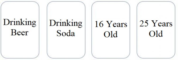
Intuitive Wason selection task: You are in charge of enforcing alcohol laws at
a bar. You will lose your job unless you enforce the following rule: If a person
drinks an alcoholic drink, then they must be at least 18 years old. The cards
below have information about four people sitting at a table in your bar. Each
card represents one person. One side of a card tells what a person is drinking,
and the other side of the card tells that person’s age. In order to enforce the law,
which of the card(s) below would you definitely need to turn over? Indicate only
those card(s) you definitely need to turn over to see if any of these people are
breaking the law.
Select the card(s) you want to turn over.
8Figure 3: Intuitive Wason task
In this “social” version (adapted from Cosmides, 1989), the correct actions are turn-
ing over the “Beer” and “16” cards. While this problem is logically the same as the ab-
stract version, previous findings show that the social context makes the problem easier
to solve.
In our experiments, each subject in the Wason condition completes both of these
tasks in randomized order. For each task, subjects can win a fixed sum of money (that
varies across treatments) if they turn over (only) the two correct cards.
2.1.3 Cognitive Reflection Test
The CRT measures people’s tendency to engage in reflective thinking (Frederick, 2005).
The test items have an intuitive, incorrect answer, and a correct answer that requires
effortful deliberation. Research has shown that people often settle on the answer that is
intuitive but wrong. We include the following two questions, both of which are widely
used in the literature:
1. A bat and a ball cost 110 KSh in total. The bat costs 100 KSh more than
the ball. How much does the ball cost? (Intuitive answer is 10, correct
answer is 5).
2. It takes 5 nurses 5 minutes to measure the blood pressure of 5 patients.
How long would it take 10 nurses to measure the blood pressure of 10
patients? (Intuitive answer is 10, correct answer is 5).
Subjects in the CRT condition complete both of these questions in randomized order.
For each question, they can earn a fixed sum of money (that varies across treatments) if
they provide exactly the correct response.
2.1.4 Anchoring
People have a tendency to use irrelevant information in making judgments. Substantial
research has shown that arbitrary initial information can become a starting point (“an-
chor”) for subsequent decisions, with only partial adjustment (Tversky and Kahneman,
91974). This can have consequential effects in situations such as negotiations, real estate
appraisals, valuations of goods, or forecasts.
To test for anchoring, we follow others in making use of a random anchor, since only
an obviously random number is genuinely uninformative. To generate a random anchor,
we ask participants for the last digit of their phone number. If this number is four or
lower, we ask them to enter the first two digits of their year of birth into the computer,
and otherwise to enter 100 minus the first two digits of their year of birth. Given that all
participants were either born in the 1900s or 2000s, this procedure creates either a low
anchor (19 or 20) or a high anchor (80 or 81). The experimental instructions clarify
that “. . . you will be asked to make estimates. Each time, you will be asked to assess
whether you think the quantity is greater than or less than the two digits that were just
generated from your year of birth.” Given these experimental procedures, the difference
in anchors across subjects is transparently random.
After creating the anchor, we ask participants to solve estimation tasks as described
below. Following standard procedures, in each task, we first ask subjects whether their
estimate is below or above the anchor. We then ask participants to provide their exact
estimate. An example sequence of questions is:
A1 Is the time (in minutes) it takes for light to travel from the Sun to the
planet Jupiter more than or less than [anchor] minutes?
A2 How many minutes does it take light to travel from the Sun to the planet
Jupiter?
where [anchor] is replaced with the random number that is generated from a partici-
pant’s phone number and year of birth. We also use three other sets of questions:
B1 In 1911, pilot Calbraith Perry Rodgers completed the first airplane trip
across the continental U.S., taking off from Long Island, New York and
landing in Pasadena, California. Did the trip take more than or less than
[anchor] days?
B2 How many days did it take Rodgers to complete the trip?
C1 Is the population of Uzbekistan as of 2018 greater than or less than [an-
chor] million?
C2 What is the population of Uzbekistan in millions of people as of 2018?
D1 Is the weight (in hundreds of tons) of the Eiffel Tower’s metal structure
more than or less than [anchor] hundred tons?
10D2 What is the weight (in hundreds of tons) of the Eiffel Tower’s metal struc-
ture?
Each of these problems has a correct solution that lies between 0 and 100. Sub-
jects are told that they can only state estimates between 0 and 100. Each participant
who takes part in the anchoring condition of our experiment completes two randomly
selected questions from the set above, in randomized order. For each question, partici-
pants can earn a fixed sum of money (that varies across treatments) if their guess g is
within g ∈ [x − 2, x + 2] for a correct response x.
2.2 Incentives and Treatment Conditions
Incentive Levels. In order to offer very high incentives and still obtain a large sample
size within a feasible budget, we conduct the experiment in a low-income country: at the
Busara Lab for Behavioral Economics in Nairobi, Kenya. For each bias, there are three
possible levels of incentives: a flat payment (no incentives), standard lab incentives, and
high incentives. With standard lab incentives, participants can earn a bonus of 130 KSh
(approx. 1.30 USD) for a correct answer. In the high incentive treatment, the size of the
bonus is multiplied by a factor of 100 to equal 13,000 KSh (approx. 130 USD).
These incentives should be compared to local living standards. Kenya’s GDP per
capita at purchasing power parity (PPP) in 2018 was $3,468, which is 18 times lower
than that of the United States. Our standard lab incentives of 130 KSh correspond to
about $23.50 at PPP in the U.S. Our high incentive condition corresponds to a potential
bonus of $2,350 at PPP in the U.S.
As a second point of comparison, we ask our student participants to provide infor-
mation on their monthly consumption and their monthly income in a post-experiment
survey. The median participant reports spending 10,000 KSh (approx. 100 USD) and
earning income of 12,000 KSh (approx. 120 USD) per month. Thus, the bonus in our
high incentive condition corresponds to 130% of median consumption and 108% of me-
dian income in our sample.
Treatments. In principle, our experiment requires three treatment conditions. How-
ever, because our primary interest is in the comparison between the standard incentive
and the high incentive conditions, we elected to implement only two treatment condi-
tions to increase statistical power.
The main experiment consists of two parts. Each participant is randomly assigned
two of the four biases. In Part 1, all participants work on tasks for the first bias in the flat
payment condition. Thus, they cannot earn a bonus in Part 1. In Part 2, they are randomly
assigned to either standard lab incentives or high incentives and complete tasks for the
11second bias. Participants only receive instructions for Part 2 after completing Part 1, and
the possibility of a bonus is never mentioned until Part 2.
With this setup, we have twice as many observations in the flat payment condition
(N = 1, 236) as in the standard lab incentive (N = 636) and high incentive (N = 600)
conditions. We keep the order of treatments constant (flat payments always followed by
standard lab incentives or high incentives), so that participants working under the flat
payment scheme are not influenced by the size of incentives in the first question.
Readers may be concerned that the comparison between the flat payment condition
and the financially incentivized conditions is confounded by order effects. We deliber-
ately accept this shortcoming. Formally, this means that a skeptical reader may only
consider the treatment comparison between standard and high incentives valid, as this
is based on randomization. Throughout the paper, we nonetheless compare the three
incentive schemes side-by-side, with the implicit understanding that our main interest
is in the comparison between standard and high incentives.
2.3 Procedures
Questions and randomization. As explained above, each bias consists of two ques-
tions. For some questions, we implement minor variations across experimental sessions
to lower the risk that participants memorize the questions and spread knowledge outside
the lab to other participants in the pool. For example, in the Wason tasks, we change
the colors of the cards from green and brown to blue and brown. To take a different
example, in the second CRT problem, we change the information from “It takes 5 nurses
5 minutes to measure the blood pressure of 5 patients” to “It takes 6 nurses 6 minutes
to measure the blood pressure of 6 patients.” Appendix B contains the full list of ques-
tions that we implement. We find no evidence that participants in later sessions perform
better than those in earlier sessions.
Each participant completes two questions in the financially incentivized part of the
experiment (Part 2). One of these two questions is randomly selected and a bonus is
given for a correct answer to that question. As explained above, for the CRT and the
Wason selection task, a participant has to give exactly the correct answer to be eligible
for a bonus. For base rate neglect and anchoring, the answer has to be within two of
the correct answer. Appendix G contains screenshots of the full experiment, including
experimental instructions and decision screens.
The stake size is randomized at the session level, mainly because the Busara Lab
was worried about dissatisfaction resulting from participants comparing their payments
to others in the same session. The set and order of the biases are randomized at the
individual level. Within each bias, we also randomize the order of the two questions.
12Salience and credibility of incentive levels. A key aspect of our design is that the stake
size is both salient and credible. We take various measures in this regard. To make the
stake size salient, the screen that introduces the second part of the experiment reads:
Part 2. We will ask you two questions on the upcoming screens. Please answer
them to the best of your ability. Please remember that you will earn a guaran-
teed show-up fee of 450 KSh. While there was no opportunity to earn a bonus in
the previous part, you will now have the opportunity to earn a bonus payment
of X KSh if your answer is correct.
where X ∈ {130; 13, 000}. The subsequent screen (which is the one that immediately
precedes the first incentivized question) reads:
Remember, you will now have the opportunity to earn a bonus payment of X
KSh if your answer is correct.²
To ensure credibility of the payments, we put in place three measures. First, we
deliberately select the Busara lab for implementation of our experiments because the
lab follows a strict no-deception rule. Second, the written instructions highlight that:
The study you are participating in today is being conducted by economists, and
our professional standards don’t allow us to deceive research subjects. Thus,
whatever we tell you, whatever you will read in the instructions on your com-
puter screen, and whatever you read in the paper instructions are all true. Ev-
erything will actually happen as we describe.
Third, the verbal instructions by Busara’s staff likewise emphasize that all information
that is provided by the experimental software is real.
Timeline. Participants are told that the experiment will last approximately one hour,
but have up to 100 minutes to complete it. This time limit was chosen based on pilots
such that it would not provide a binding constraint to participants; indeed no partici-
pants use all of the allotted time. The timeline of the experiment is as follows: (i) elec-
tronic consent procedure; (ii) general instructions; (iii) two unincentivized questions
in Part 1; (iv) screen announcing the possibility of earning a bonus in Part 2; (v) two
financially incentivized questions in Part 2; and (vi) a post-experimental questionnaire.
Screenshots of each step are provided in Appendix G.
²To further verify participant understanding and attention, the post-experimental survey includes
non-incentivized questions that ask subjects to recall the possible bonus amounts in Parts 1 and 2. Tables 14
and 15 show that our results are very similar when we restrict the sample to those tasks for which a subject
recalls the incentive amount exactly correctly (64% of all data points). This is arguably a very conservative
procedure because (i) a large majority of subjects recall incentive amounts that are in the ballpark of the
correct answer, and (ii) subjects might be aware of the exact stake size when solving the problems, but
might not remember the precise amounts later.
13Earnings. Average earnings are 482 KSh in the standard incentive condition and 3,852
KSh in the high incentive condition. This includes a show-up fee of 450 KSh. Per the
standard procedure of the Busara Lab, all payments are transferred electronically within
24 hours of participation.
2.4 Participants
The experimental sessions take place at the Busara Center for Behavioral Economics
in Nairobi, Kenya. We conduct our experiments in this lab due to the lab’s capabilities
in administering experiments without deception as well as the lab’s ability to recruit a
large number of analytically capable students for whom our large incentive treatment is
equal to approximately a month’s worth of their consumption. Participants are recruited
among students of the University of Nairobi, the largest public university in Kenya. Ta-
ble 1 reports the resulting sample sizes by bias and incentive level.³ In total, 1,236 par-
ticipants completed the study between April and July 2019. The majority (93 percent)
are between 18 and 24 years old (mean age 22) and 44 percent are female.
It may be helpful to compare the level of cognitive skills in our sample with that
of more traditional subject pools used in the United States. The two CRT questions in
our study are part of the three-question module for which Frederick (2005) reports
summary statistics across various participant pools. In the no incentive condition of our
experiments at Busara, 34% of all CRT questions are answered correctly. In Frederick’s
review, the corresponding numbers are, inter alia, 73% at MIT; 54% at Princeton; 50%
at CMU; 48% at Harvard; 37% in web-based studies; 28% at University of Michigan
Dearborn; 26% at Michigan State; and 19% at Toledo University.⁴ Thus, according to
these metrics, our subject pool has lower average performance scores than the most
selective U.S. universities, but it compares favorably with participants from more typical
U.S. schools.⁵
³Table 5 in Appendix D reports summary statistics for participant characteristics across treatments.
⁴We report averages for the entire three-question module from Frederick (2005). While we only use
the first two questions of his module at Busara, we are not aware of evidence that the module’s third
question is substantially harder than the other two.
⁵A second, and perhaps more heuristic, comparison is to follow Sandefur (2018), who recently de-
vised a method to construct global learning metrics by linking regional and international standardized
test scores (such as TIMSS). His data suggest that Kenya has some of the highest test scores in his
sample of 14 African countries. He concludes that “the top-scoring African countries produce grade 6
scores that are roughly equivalent to grade 3 or 4 scores in some OECD countries.” Of course, this com-
parison is only heuristic because (i) it pertains to primary school rather than college students and (ii)
it ignores the (likely highly positive) selection of Kenyan students into the University of Nairobi. In-
deed, the University of Nairobi is the most prestigious public university in Kenya and routinely ranks
as the top university in the country and among the top universities in Africa. See, for example, https:
//www.usnews.com/education/best-global-universities/africa?page=2.
14Table 1: Number of participants by bias and incentive level
No incentives Standard incentives High incentives
Base rate neglect 309 159 150
Contingent reasoning 308 160 151
CRT 311 163 146
Anchoring 308 154 153
Total 1,236 636 600
2.5 Pre-Registration and Hypotheses
We pre-registered the design, analysis, and target sample size on www.aspredicted.org at
https://aspredicted.org/blind.php?x=5jm93d. The pre-registration specified an
overall sample size of 1,140 participants, yet our final sample consists of 1,236 partic-
ipants. We contracted with the Busara lab not for a total sample size, but for a total
amount of money that would have to be spent. Thus, our target sample size was based
on projections of how costly the experiment would be, in particular on a projection of the
fraction of subjects that would earn the bonus in the high incentive condition. Because
it turned out that slightly fewer subjects earned the bonus than we had anticipated,
there was still “money left” when we arrived at 1,140 participants. Busara gave us a
choice between forfeiting the money and sampling additional participants, and – being
efficiency-oriented economists – we elected to sample additional subjects to increase sta-
tistical power. Tables 8 and 9 in Appendix D replicate our main results on a sample of
the first 1,140 participants only. The results are very similar.⁶
The pre-registration specified three types of hypotheses. First, across all tasks, we pre-
dicted that response times would monotonically increase as a function of the stake size.
Response times are a widely used proxy for cognitive effort in laboratory experiments
(Rubinstein, 2007, 2016; Enke and Zimmermann, 2019). Because each question is pre-
sented in a self-contained manner on a separate screen (including the question-specific
instructions), we have precise and meaningful data on response times.
Second, we predicted that performance would monotonically improve as a function
of the stake size for the following tasks: intuitive base rate neglect, intuitive Wason,
CRT, and anchoring. Third, we predicted that performance would not change across
incentive levels for abstract base rate neglect and abstract Wason. The reasoning behind
these differential predictions is that the more abstract versions of base rate neglect and
⁶The only difference in results is that in the high stakes condition of the intuitive BRN task, the
performance improvement relative to the standard incentives condition is statistically significant at the
10% level in this sample, though the effect size is small and comparable to what is reported in the main
text below.
15the Wason selection task may be so difficult conceptually that even high cognitive effort
does not generate improved responses.
2.6 Expert Predictions
To complement our pre-registration and to be able to compare our results with the profes-
sion’s priors, we collect expert predictions for our experiments (Gneezy and Rustichini,
2000; DellaVigna and Pope, 2018). In this prediction exercise, we supply forecasters
with average response times and average performance for each bias in the absence of
incentives, using our own experimental data. Based on these data, we ask our experts
to predict response times and performance in the standard incentive and high incentive
conditions. Thus, each expert issues 24 predictions (six tasks times two treatments times
two outcome variables). Experts are incentivized in expectation: we paid $100 to the
expert who issued the set of predictions that turned out to be closest to the actual data.
The expert survey can be accessed at https://hbs.qualtrics.com/jfe/form/SV_
bDVhtmyvlrNKc6N.
Our total sample of 68 experts comprises a mix of experimental economists and Har-
vard students with graduate-level exposure to experimental economics. First, we con-
tacted 231 participants of a recent conference of the Economic Science Association (the
professional body of experimental economists) via email. Out of these, 45 researchers
volunteered to participate in our prediction survey, 41 of which self-identified with Ex-
perimental Economics as their primary research field in our survey. In addition, we con-
tacted all students who had completed Enke’s graduate experimental economics class
at Harvard in 2017–2019, which produced 23 student volunteers. The predictions of
professionals and Harvard students turn out to be similar, on average.⁷ We hence pool
them for the purpose of all analyses below.⁸
3 Results
3.1 Summary Statistics on Frequency of Cognitive Biases
A prerequisite for our study to be meaningful is the presence of cognitive biases in our
sample. This is indeed the case. Appendix C summarizes the distribution of responses
⁷Professional experimental economists tend to predict slightly smaller increases in response times and
performance as a function of stakes, but these differences are rarely statistically significant.
⁸The experts appear to exhibit a meaningful level of motivation. In our survey, we only briefly describe
the study by providing the names of the experimental tasks. In addition, we provide the experts with an
option to view details on the implementation of these tasks. Across the six different tasks, 53%-84% of
experts elect to view the task details, with an overall average of 68%. Of course, some experts may not
need to look up the task details because they know the task structure.
16for each of our tasks, pooled across incentive conditions.
In the CRT, 39% of responses are correct. As shown in Figure 8 in Appendix C, about
50% of all answers correspond exactly to the well-known “intuitive” response.
In the abstract base rate neglect task, 11% of all responses are approximately correct
(defined as within 5 percentage points of the Bayesian posterior); the corresponding
number is 26% for the intuitive version. Across all base rate neglect tasks, we see that
subjects’ responses tend to be too high, effectively ignoring the low base rate. See Fig-
ure 9 in Appendix C.
In the Wason selection task, 14% of responses are correct in the abstract frame and
57% in the intuitive frame. This level difference is consistent with prior findings. As
documented in Appendix C, a common mistake in Wason tasks of the form A ⇒ B is to
turn over “B” rather than “not B”.
In the anchoring tasks, we find statistically significant evidence of anchoring on ir-
relevant information. Across questions, the correlations between subjects’ estimates and
the anchors range between ρ = 0.38 and ρ = 0.60. Figure 10 in Appendix C shows the
distributions of responses as a function of the anchors.
In summary, pooling across incentive conditions, we find strong evidence for the
existence of cognitive biases, on average. We now turn to the main object of interest of
our study, which is the effect of financial incentives.
3.2 Incentives and Effort
We start by examining whether higher stakes induce participants to increase effort, using
response time as a proxy for effort. This analysis can plausibly be understood as a “first
stage” for the relationship between incentives and cognitive biases. In absolute terms,
average response times range from 99 seconds per question in anchoring to 425 seconds
per question in intuitive base rate neglect, which includes the time it takes participants
to read the (very short) instructions on their decision screens.
Figure 4 visualizes mean response times by incentive level, separately for each ex-
perimental task. Here, to ease interpetation, response times are normalized to one in
the no incentives condition. In other words, for each cognitive bias, we divide observed
response times by the average response time in the no incentives condition. Thus, in
Figure 4, response times can be interpreted as a percentage of response times in the no
incentives condition.
We find that standard lab incentives generally do not increase response times much
compared to no incentives. High incentives, however, robustly lead to greater effort,
a pattern that is very similar across all tasks. Overall, response times are 39 percent
higher in the high incentive condition compared to standard incentives. We observe the
17Cognitive Reflection Test Base rate neglect
1.6 1.6
Normalized response time
Normalized response time
1.4 1.4
1.2 1.2
1 1
.8 .8
No incentives Standard incentives High incentives No incentives Standard incentives High incentives
CRT Abstract BRN Intuitive BRN
Contingent reasoning Anchoring
1.6 1.6
Normalized response time
Normalized response time
1.4 1.4
1.2 1.2
1 1
.8 .8
No incentives Standard incentives High incentives No incentives Standard incentives High incentives
Abstract Wason Intuitive Wason Anchoring
Figure 4: Average normalized response times across incentive conditions. Response times are normalized
relative to the no incentive condition: for each cognitive bias, we divide observed response times by the
average response time in the no incentive condition. Error bars indicate +/- 1 s.e.
largest increase (52 percent) in intuitive base rate neglect, and the smallest increase
(24 percent) in anchoring. Figure 12 in Appendix E shows that very similar results hold
when we look at median response times.
Table 2 quantifies the effects of incentive size on response times (in seconds) using
OLS regressions.⁹ In these regressions, the omitted category is the standard incentive
condition. Thus, the coefficients of the no incentive and the high incentive conditions
identify the change in response times in seconds relative to the standard incentive con-
dition. The last row of the table reports the p-value of a test for equality of regression
coefficients between No incentives and High incentives, although again this comparison
is not based on randomization. For each subject who worked on a given bias, we have
two observations, so we always cluster the standard errors at the subject level.
Perhaps with the exception of the anchoring tasks, we can never reject the hypothesis
that cognitive effort in the flat payment and standard incentive schemes are identical.
In fact, the estimated coefficient is sometimes positive and sometimes negative. While
⁹Table 6 in Appendix D provides complementary nonparametric tests that deliver very similar results.
18Table 2: Response times across incentive conditions
Dependent variable:
Response time [seconds]
Omitted category: Base rate neglect Contingent reasoning
Standard incentives CRT Abstract Intuitive Abstract Intuitive Anchoring
(1) (2) (3) (4) (5) (6)
1 if No incentives 2.16 -4.71 19.5 -12.7 0.28 -10.2∗
(10.25) (20.51) (24.79) (7.72) (4.72) (6.14)
1 if High incentives 55.5∗∗∗ 141.6∗∗∗ 190.7∗∗∗ 52.4∗∗∗ 29.2∗∗∗ 23.6∗∗
(14.63) (33.55) (41.17) (13.21) (6.43) (9.88)
Constant 157.2∗∗∗ 303.1∗∗∗ 368.8∗∗∗ 174.5∗∗∗ 105.9∗∗∗ 97.8∗∗∗
(7.94) (15.77) (16.74) (6.31) (3.64) (5.44)
Observations 1240 618 618 619 619 1230
R2 0.02 0.05 0.05 0.07 0.05 0.03
p-value: No inc. = High inc. < 0.01 < 0.01 < 0.01 < 0.01 < 0.01 < 0.01
Notes. OLS estimates, standard errors (clustered at subject level) in parentheses. Omitted category:
standard incentive scheme. The last row reports the p-value of a test for equality of regression
coefficients between No incentives and High incentives. ∗ p < 0.10, ∗∗ p < 0.05, ∗∗∗ p < 0.01.
it should be kept in mind that the coefficient of the no incentive condition is potentially
confounded by order effects, we still view this result as suggestive.
High stakes, on the other hand, significantly increase response times by between 24
seconds (anchoring) and 191 seconds (intuitive base rate neglect), relative to the stan-
dard incentive treatment. Indeed, as we show in Figure 11 in Appendix E, the empirical
cumulative distribution functions of response times in the high incentive conditions usu-
ally first-order stochastically dominate the CDFs in the other conditions.¹⁰
Even though in relative terms high stakes induce a substantial increase in response
times, the rather modest increase in absolute response times is noteworthy, given the
large increase in financial incentives. Potential explanations for this – which we cannot
disentangle – are the presence of substantial cognitive effort costs, overconfidence, or a
belief that more cognitive effort does not improve performance on the margin.
Result 1. Very high incentives increase response times by 24–52% relative to standard lab
incentives. Response times are almost identical with standard incentives and no incentives.
3.3 Incentives and Cognitive Biases
Figure 5 shows how variation in the stake size affects the prevalence of our cognitive
biases. For the CRT, base rate neglect, and the Wason selection task, the figure shows
¹⁰Table 10 in Appendix D shows that results are robust to controlling for individual characteristics and
question fixed effects.
19the fraction of correct answers. For base rate neglect, following our pre-registration, we
count a response as “correct” if it is within 5 percentage points of the Bayesian posterior.
While subjects only received a bonus if their answer was within 2 percentage points of
the Bayesian response, we work here with a slightly larger interval to allow for random
computational errors.¹¹ For anchoring, we plot one minus the Pearson correlation co-
efficient between responses and the anchor, so that higher values reflect less cognitive
bias.
The main takeaway is that performance barely improves. In the CRT, performance
in the high incentive condition increases by about 10 percentage points relative to the
standard incentive condition. However, in all other tasks, improvements are either very
small or entirely absent. Across all tasks, high incentives never come close to eradicating
the behavioral biases. These results suggest that judgmental biases are not an artifact
of weak incentives.
Table 3 quantifies these results through regression analysis.¹² Here, in columns (1)–
(5), the dependent variable is whether a given task was solved correctly. In the first
five columns, the coefficients of interest are the treatment dummies. Again, the omitted
category is the standard incentive condition.
For anchoring, column (6), the object of interest is not whether a subject’s answer
is objectively correct, but instead how answers vary as a function of the anchor. Thus,
the coefficients of interest are the interactions between the anchor and the treatment
dummies.
Compared to standard incentives, flat payments appear to have virtually no effect
on performance in all problems, perhaps with the exception of the abstract Wason task.
High stakes, on the other hand, lead to a statistically significant increase in performance
on the CRT. For intuitive base rate neglect, the intuitive Wason task, and anchoring, the
estimated coefficients of interest are positive but not statistically significant. For abstract
base rate neglect and the abstract Wason task, the point estimates are even negative.¹³
In quantitative terms, the improvements in performance are modest. Importantly,
the weak effects of the large increase in financial incentives are not driven by a lack of
statistical power. Given our large sample size, the regression coefficients are relatively
tightly estimated. Looking at 95% confidence intervals, we can rule out that, going from
standard to high incentives, performance increases by more than: 18 pp in the CRT, 4
¹¹Results are very similar if we use (i) absolute distance between the response and the Bayesian pos-
terior as a continuous performance measure, or (ii) a binary performance measure with a band of 2
percentage points around the Bayesian posterior. See Table 12 in Appendix D.
¹²Table 7 in Appendix D provides complementary nonparametric tests that deliver very similar results.
¹³Table 11 in Appendix D shows that controlling for individual characteristics and question fixed ef-
fects leaves the results unaffected. We also conduct heterogeneity analyses with respect to college GPA,
score on a Raven matrices test (a measure of intelligence), and income. We find no robust evidence of
heterogeneous treatment effects along these dimensions.
20You can also read