Complete phase retrieval of photoelectron wavepackets
←
→
Page content transcription
If your browser does not render page correctly, please read the page content below
PAPER • OPEN ACCESS

Complete phase retrieval of photoelectron wavepackets
To cite this article: L Pedrelli et al 2020 New J. Phys. 22 053028

View the article online for updates and enhancements.

                                This content was downloaded from IP address 46.4.80.155 on 18/09/2021 at 10:01
New J. Phys. 22 (2020) 053028                                                                https://doi.org/10.1088/1367-2630/ab83d7

                                 PAPER

                                 Complete phase retrieval of photoelectron wavepackets
O P E N AC C E S S

R E C E IVE D
                                 L Pedrelli1 , 4 , P D Keathley2 , 4 , L Cattaneo1 , F X Kärtner2 , 3 and U Keller1
16 December 2019                 1
                                     Physics Department, Institute of Quantum Electronics, ETH Zürich, 8093 Zürich, Switzerland
                                 2
R E VISE D                           Research Laboratory of Electronics, Massachusetts Institute of Technology, Cambridge, MA 02139, United States of America
25 March 2020                    3
                                     Center of Free-Electron Laser Science, DESY and Department of Physics, University of Hamburg, D-22607 Hamburg, Germany
                                 4
AC C E PTE D FOR PUBL IC ATION       L Pedrelli and P D Keathley contributed equally to this work.
26 March 2020
                                 E-mail: lucaped@phys.ethz.ch
PUBL ISHE D
19 May 2020                      Keywords: attosecond science, strong-field physics, atomic, optical and molecular physics, ultrafast science

                                 Supplementary material for this article is available online
Original content from
this work may be used
under the terms of the
Creative Commons
Attribution 4.0 licence.         Abstract
Any further distribution         Coherent, broadband pulses of extreme ultraviolet light provide a new and exciting tool for
of this work must
maintain attribution to          exploring attosecond electron dynamics. Using photoelectron streaking, interferometric
the author(s) and the
title of the work, journal
                                 spectrograms can be generated that contain a wealth of information about the phase properties of
citation and DOI.                the photoionization process. If properly retrieved, this phase information reveals attosecond
                                 dynamics during photoelectron emission such as multielectron dynamics and resonance processes.
                                 However, until now, the full retrieval of the continuous electron wavepacket phase from isolated
                                 attosecond pulses has remained challenging. Here, after elucidating key approximations and
                                 limitations that hinder one from extracting the coherent electron wavepacket dynamics using
                                 available retrieval algorithms, we present a new method called absolute complex dipole transition
                                 matrix element reconstruction (ACDC). We apply the ACDC method to experimental
                                 spectrograms to resolve the phase and group delay difference between photoelectrons emitted
                                 from Ne and Ar. Our results reveal subtle dynamics in this group delay difference of
                                 photoelectrons emitted form Ar. These group delay dynamics were not resolvable with prior
                                 methods that were only able to extract phase information at discrete energy levels, emphasizing the
                                 importance of a complete and continuous phase retrieval technique such as ACDC. Here we also
                                 make this new ACDC retrieval algorithm available with appropriate citation in return.

                                 1. Introduction

                                 When high-energy photons interact with a gas target, photoelectrons are generated. While the rate of this
                                 photoelectron generation can be described by the gas species’ cross-section, the attosecond dynamics of the
                                 emission process are more difficult to resolve [1–3]. Revealing these dynamics is a key challenge to
                                 understanding multi-electron interactions and resonant processes occurring in any system more
                                 complicated than the hydrogen atom [4–7]. However, the accurate characterization of photoionization
                                 dynamics requires the phase information acquired by the electron wavepacket during the transition from
                                 the ground state to the excited state in the ionization process.
                                     There has been a large amount of interest in characterizing this phase information in the past years via
                                 reconstruction of attosecond beating by interference of two-photon transitions (RABBITT) [8, 9] or via a
                                 fully optical interferometric technique [10] which requires the use of discrete harmonics of an attosecond
                                 pulse train. Such methods lead to a coarse energy sampling and cannot resolve fast oscillations in the group
                                 delay as a function of energy. Recently, there has been interest in the analysis of continuous spectrograms
                                 from isolated attosecond pulses to increase the energy resolution of the relative phase of the emitted
                                 electron wavepackets [2, 3, 11, 12]. However, these methods are still encumbered by many approximations
                                 that limit their overall effectiveness.
                                     In this work, we develop a new method for the complete characterization of photoelectron wavepackets
                                 using photoelectron streaking spectrograms from isolated attosecond pulses which we call absolute complex

                                 © 2020 The Author(s). Published by IOP Publishing Ltd on behalf of the Institute of Physics and Deutsche Physikalische Gesellschaft
New J. Phys. 22 (2020) 053028                                                                      L Pedrelli et al

dipole transition matrix element reconstruction (ACDC). The ACDC method is not limited by any
approximation other than the strong-field approximation (SFA) used to model the photoionization and
streaking process, enabling unprecedented accuracy in the retrieval of the photoelectron wavepacket’s phase
across a continuous spectrum of electron energies. Applying ACDC to simultaneously measured
photoelectron streaking spectrograms from Ar and Ne, we reveal subtle dynamics in the group delay of the
photoionization process from Ar that would have been impossible to resolve using prior techniques that
sampled the group delay at discrete energy points.
    This paper is structured as follows. In section 2 we start with an overview of phase-retrieval techniques
and their application in phase and group delay analysis of photoelectron wavepackets. In section 3 we
introduce and briefly review the so-called wavepacket approximation [11, 13], that prevents conventional
attosecond pulse characterization algorithms from accurately retrieving the complete electron wavepacket
from streaking spectrograms. In section 4, we introduce the ACDC method, demonstrating its capability of
overcoming the wavepacket approximation to fully characterize electron wavepackets and attosecond time
delays in photoemission to within the limits of the SFA. Finally, in section 5, we use the ACDC method to
reconstruct the dipole phase of electron wavepackets excited from Ar using experimental streaking
measurements.
    Our results agree very well with the average group delay measurements using discrete harmonics [10],
showing almost a π shift in phase at photon energies ranging from 26 to 30 eV, corresponding to the energy
position of the well-known 3s3p6 np autoionizing series of Ar [14]. Furthermore, the ACDC reconstruction
reveals new group-delay features between 30 and 35 eV that could not be resolved by other techniques. Our
results emphasize the importance of the complete and continuous phase retrieval method we use here. We
believe that, this work opens the door to more complex studies such as photoelectron excitation dynamics
in molecular systems.

2. Extreme-ultraviolet phase retrieval techniques for photoelectron wavepacket
analysis

To experimentally investigate attosecond photoemission dynamics, two methods are commonly used: (1)
RABBITT [8, 9]; and (2) the photoelectron streaking from single attosecond pulses (SAPs) [15]. Both
techniques employ a pump–probe scheme, where an extreme-ultraviolet (XUV) attosecond pump pulse
initiates electron dynamics and an infrared (IR) probe pulse interrogates the temporal evolution of the
released electrons as the delay τ between pump and probe is varied. While the RABBITT technique uses an
attosecond pulse train (APT) in combination with a weak (
New J. Phys. 22 (2020) 053028 L Pedrelli et al
Figure 1. Scheme of the experimental setup including the COLTRIMS detector used to simultaneously measure the streaking
spectrograms of Ne (top) and Ar (bottom) considered in this work. The red line represents the path of the IR beam which is
spited in two parts by the beam splitter (BS). 80% is used to generate, using the polarization gating (PG) scheme, the XUV pump
beam (EXUV ) while the remaining 20% is used as the probe streaking field (EIR ). The scheme of the experimental setup has been
adapted from [19].
where ϕXUV is the attochirp phase of the SAP, ϕW is the Wigner phase and ϕCLC is the Coulomb-laser
coupling phase which takes into account the extra phase that the photoemitted electron wavepacket acquires
due to the interaction with both the long-range Coulomb potential and the IR streaking field, very similar
to the continuum–continuum phase in the RABBITT technique [17].
The derivative of the retrieved spectral phase ϕstk (E) corresponds to the group delay (GD) of the excited
electron wavepacket, i.e.
∂ϕstk (E)
GD = . (2)
∂E
The attochirp contribution to ϕstk can be eliminated by computing the GD difference between two
different species measured simultaneously and subject to the same ionizing XUV spectrum. This requires
the use of a coincidence detection apparatus such as the cold target recoil ion momentum spectrometer
(COLTRIMS) [18]. Experimental streaking spectrograms measured simultaneously in Ar and Ne using the
COLTRIMS apparatus [19] and which will be object of our analysis in section 5 of this work are shown in
figure 1.
The measurement-induced contribution ϕCLC can be extracted from numerical calculation [20] such
that by comparison of two simultaneously measured streaking spectrograms the extracted phase has only
the Wigner contribution. However, as alluded to earlier, access to ϕW (E) from photoelectron streaking
measurements requires a numerical retrieval algorithm.
Frequency resolved optical gating for complete retrieval of attosecond bursts (FROG-CRAB) [21, 22] is a
well-established and widely used method for characterizing the time-domain profile of XUV pulses (both
amplitude and phase) from streaking spectrograms. A critical analysis in retrieving the phase of the
photoemitted electron wavepacket using FROG-CRAB methods has been carried out by Wei et al [1] where
they point out limitations of the method, namely the central momentum approximation and what they call
the wavepacket approximation (WPA) [11, 13]. In their work, they were unable to overcome these
limitations to fully recover the phase of the photoelectron wavepacket. While others have shown the ability
to circumvent the central-momentum approximation [23], to our knowledge the wavepacket
approximation remains the limiting factor in accurate photoelectron retrieval. In the following sections, we
define the wavepacket approximation and demonstrate why it is so problematic. We then present the ACDC
method which overcomes the wavepacket approximation and use it with the experimental data shown in
figure 1 to reveal newly observed group-delay dynamics in photoemission from Ar.
3. Wavepacket approximation (WPA)
The complex amplitude of a photoelectron going from the ground state to the final state with momentum k
can be expressed within the SFA
+∞
k2
iφ(k,t) i IP + 2 t
ãSFA (k, τ ) = −i dt d̃ (k + A (t)) ẼXUV (t − τ )e e , (3)
−∞
3New J. Phys. 22 (2020) 053028 L Pedrelli et al
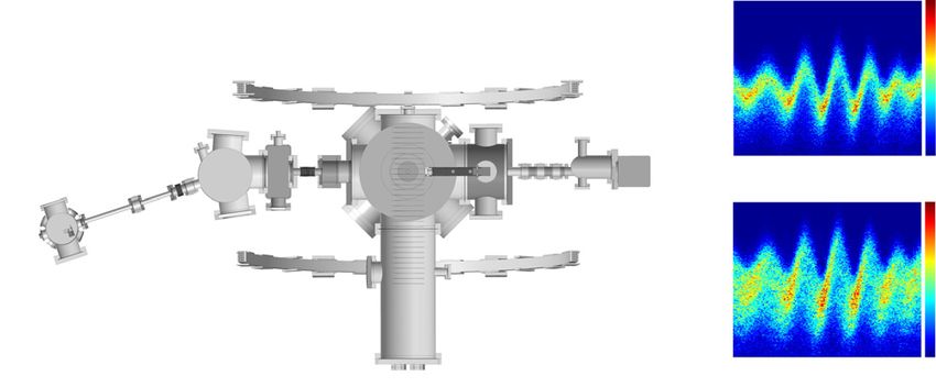
Figure 2. Simulated streaking spectrograms using (a) the SFA model SSFA (k, τ ) = |ãSFA (k, τ )|2 and (b) using the WPA, i.e.
SWPA (k, τ ) = |ãWPA (k, τ )|2 . We observe a percentage difference between the two spectrograms shown here of up to 35% mainly
concentrated around the central energy of the spectrogram.
where d̃(k) is the dipole transition matrix element (DTME), τ the time delay between the XUV pump pulse
and the IR probe pulse, ẼXUV (t) is the XUV field in time domain and A(t) the vector potential of the IR
electric field from which it can be calculated, EIR (t) = − ∂t∂ A(t).
The phase modulation term, φ(k, t), resulting from the accumulated phase of the electron during the
streaking process reads
+∞
1 2
φ (k, t) = − dt kA t + A (t ) . (4)
t 2
The measured photoelectron spectrum is given by the probability of measuring an electron with
momentum k and delay τ , i.e. SSFA (k, τ ) = |ãSFA (k, τ )|2 .
In absence of the IR electric field, the XUV pulse, ionizing the target gas, generate a photoelectron
wavepacket that can be expressed in the energy domain as
k2
χ̃ (E) = ẼXUV IP + d̃(E). (5)
2
Introducing the expression of the wavepacket (5) into equation (3) we can rewrite the SFA complex
amplitude within the WPA as follows
+∞
k2
iφ(k,t) i IP + 2 t
ãWPA (k, τ ) = −i dt χ̃ (t − τ ) e e . (6)
−∞
As explained in [11], the WPA is not an exact theory but rather an approximation to the SFA model
given by equation (3), which is considered the model better describing the physics of the streaking process.
The difference between the spectrogram SSFA (k, τ ) and SWPA (k, τ ) = |ãWPA (k, τ )|2 can be seen by comparing
SSFA and SWPA as we show in figure 2.
Most photoelectron retrieval methods based on FROG-CRAB, when used to characterize the electron
wavepacket χ̃ (E), rely on the WPA (i.e. they use ãWPA to model the streaking process rather than ãSFA ),
which leads to significant errors in the retrieved phase response and group delay as the physics of the
experiment is better described by ãSFA [see appendix A for further analysis (http://stacks.iop.org/NJP/22/
053028/mmedia)]. In the following sections, we introduce the ACDC method which overcomes the WPA,
enabling a complete characterization of the photoemitted electron wavepacket.
4. Absolute complex DTME reconstruction (ACDC) algorithm
In this section we describe the method of the ACDC algorithm to retrieve the DTME (d̃), when both the
XUV and IR pulses are known quantities.
Starting from the SFA expression of the complex amplitude of the photoemitted electron wavepacket
given by equation (3), we now approximate d̃ using the first order Taylor expansion at such that
d̃ (k + A(t + τ )) ≈ d̃ (k) + d̃ (k)A(t + τ ), (7)
where d̃ (k) = ∂k d̃. In this way we can rewrite the complex amplitude describing the transition from the
ground state to the final momentum k as:
ãSFA (k, τ ) ≈ d̃ (k) Γ̃(k, τ ) + d̃ (k)β̃(k, τ ) (8)
4New J. Phys. 22 (2020) 053028 L Pedrelli et al
where we introduced
+∞ 2
i IP t + k2 t
Γ̃ (k, τ ) = −i dt ẼX (t)eiφ(k,t +τ ) e (9)
−∞
and
+∞ k2 t
iφ(k,t +τ ) i IP t + 2
β̃ (k, τ ) = −i dtA (t + τ ) ẼX (t) e e . (10)
−∞
When we numerically sample the momentum and time delay components, we approximate the
derivative of d̃ as:
d̃ [m + 1] − d [m − 1]
d̃ [m] = (11)
Δk[m]
where m is the sample number in energy and Δk [m] = k [m + 1] − k[m − 1]. Using this we can write
d̃ [m + 1] β̃ [l, m] d̃ [m − 1] β̃[l, m]
ãSFA [l, m] = d̃ [m] Γ̃ [l, m] + − (12)
Δk [m] Δk[m]
where l is the sample number of time delays.
Using the same minimization strategy as Volkov transform generalized projections algorithm (VTGPA)
[23] we define the matrix ã [l, m] as
ã [l, m] = P[l, m]ei arg(ãSFA [l,m]) (13)
that is the measured spectrogram amplitude P [l, m] projected onto the computed spectrogram ãSFA [l, m].
From this we can define the figure of merit M
M= ãSFA [l, m] − ã [l, m] × c · c (14)
l m
and the value of d̃[m] = d[m]eiφ[m] that minimizes M by solving the system of equations
∂M ∂M
= 0; = 0. (15)
∂d [m] ∂φ [m]
In appendix B we report the full derivation of the expression of d̃.
For low streaking intensities (1 × 10¹⁰ W cm−2 ), this approach accurately reconstructs d̃ (see
simulation results in appendix B). However, when the streaking intensity, and thus the streaking vector
potential, is large (>1 × 10¹⁰ W cm−2 ), the Taylor expansion used in equation (7) becomes inadequate.
Expanding to higher orders was found to be overly cumbersome, and in the end the most effective approach
in this case was to: (1) use the analytical method described above using the first order Taylor expansion as a
first step to estimate the amplitude and phase of d̃; and (2) apply a numerical stochastic gradient descent
algorithm to refine the estimated DTME from (1), bringing it much closer to the actual solution.
For step (2), we used a stochastic gradient descent algorithm along with Adam (adaptive momentum
estimation) optimizer [24]. The use of step (1) is justified by the fact that, the convergence to local minima
of the cost function, when using the step (2), results faster.
For simplicity, we leave the technical description, together with the effect of the approximation of the
first order Taylor expansion, in appendix B. Additionally, in appendix C we show the robustness of the
ACDC method on simulated spectrograms using different streaking parameters, i.e. IR intensity, XUV
bandwidth and XUV chirp.
In figure 3, we show the result of the ACDC method when reconstructing a simulated spectrogram from
Ar. Artificial Poisson noise was added to the simulated spectrogram to mimic the noise observed in the
experimental data (figure 1).
Since we want to reconstruct the DTME from experimental spectrograms, we also considered
parameters of both the XUV and the IR field similar to the experimental conditions that we will consider in
the next section. In particular, we used an IR intensity of 3 × 10¹² W cm−2 while the XUV spectrum (grey
shaded area in figure 3) resembles the actual spectrum used during experiments. The red line in figure 3
represents the reconstructed GD using the ACDC method in absence of noise while the green curve shows
the result in presence of noise level comparable to the experiment (see appendix D for details of noise
analysis).
Despite the fact that fluctuations due to noise are still present, we observe a good agreement with the
theoretical curve used as the input for the GDAr (black line) [3] over the entire energy window considered
for the reconstruction, including the rapid group delay fluctuations from 34–38 eV. This result validates the
algorithm’s robustness against noise and its applicability to experimental measurements which is considered
in the next section.
5New J. Phys. 22 (2020) 053028 L Pedrelli et al
Figure 3. (a) Simulated streaking spectrogram with a Poisson noise level comparable to the experimental conditions. (b)
Retrieved GD with ACDC without noise (red line) and in presence of noise (green line). The green line is the weighted average of
19 reconstructions on different pump probe delay windows of 2 fs. The theory curve (black line) used as input to generate the
simulated spectrogram shown in (a) is from reference [3]. In order to be able to simulate the spectrograms avoiding unphysical
abrupt jumps in the simulated spectrogram amplitude, we extended the theoretical curve below 27.8 eV and above 40.5 eV (black
dashed lines). The grey shaded area shows the XUV spectral intensity reproducing the experimental case.
5. Experimental reconstruction of the Ar dipole phase
In this section we retrieved the dipole phase of Ar from the experimental spectrogram shown in figure 1
using ACDC. In figure 4 the blue line and blue shaded area show the reconstructed Ar dipole phase
resulting from 36 averages using the ACDC algorithm and its standard deviation, respectively. For the
interested reader, the details of the reconstruction procedure can be found in appendix E.
The dipole phase difference between Ne and Ar have also been measured experimentally by Azoury et al
using optical attosecond interferometry [10]. Adapting their result by flipping the sign and adding the Ne
dipole phase from reference [25] (yellow squares in figure 4), we observe an excellent agreement with the
ACDC reconstruction over the full energy spectrum. However, since the ACDC algorithm resolves the phase
in a continuous manner, a much finer phase structure is resolved as a function of photon energy.
In the present measurement we sampled the Ar DTME every 0.15 eV, while in [10] it was every ∼3.1 eV
due to the spacing of the discrete XUV harmonics.
The ACDC result reveals a pronounced peak in the dipole phase of Ar between 30 to 32 eV [label (b) in
figure 4] and a subsequent dip in the energy region from 33 to 35 eV [label (c) in figure 4] which cannot be
described by a piecewise linear fit between the data points from [10].
In order to compare the obtained GDAr with the differential group delay ΔGDArNe reported from other
experiments, we subtracted the GD of Ne from GDAr using the theoretical calculation from reference [25].
The result is shown in figure 5 by the blue curve together with the blue shaded region, which represents the
standard deviation. We note the persistent rapid variations of the ΔGDArNe that lie in the energy region
where the Ar autoionizing states are located as displayed by the black vertical lines. While these oscillations
are intriguing, they are near the noise limits of the retrievals from our current measurement data, and to
fully confirm that those oscillations are signature of the 3s3p6 np autoionizing states will require further
investigations that go beyond the scope of this work.
In figure 5 we also plot several data points from previously reported RABBITT-like measurements of the
average group delay ΔGDArNe (green, blue and grey squares [2], magenta circles [26], and yellow
6New J. Phys. 22 (2020) 053028 L Pedrelli et al
Figure 4. The blue curve displays the average of 36 retrieved Ar dipole phases from the reconstruction of experimental
measurement using the ACDC algorithm. The yellow symbols are adapted experimental result from reference [10] and shifted to
within a constant offset. The labels (a)–(c) refer to the discussion in the main text.
Figure 5. Retrieved ΔGDArNe from experimental streaking measurement using the ACDC algorithm averaging 36
reconstructions is shown by the blue curve together with its standard deviation (blue shaded area). RABBITT measurements
from reference [2] (green, blue and grey squares) and from reference [26] (magenta circles) are displayed. Results from a fully
optical interferometric technique from reference [10] are also plotted with yellow squares. The black vertical lines show the
calculated 3s3p6 np autoionizing series of Ar from reference [14].
squares [10]). We observe that, between 28 to 30 eV the ACDC result retrieves, on average, a higher
ΔGDArNe compared to RABBITT measurements while, between 30 to 34 eV, the ACDC result predicts a
lower value. These correspond to the regions labelled as (a)–(c) in figure 4. This discrepancy between
ΔGDArNe retrieved by ACDC and the RABBITT measurements arises due to the ACDC’s ability to more
finely sample the phase of the DTME. Indeed, the comparison between the ΔGDArNe curve reconstructed
with the ACDC from the SAP streaking measurement and the other data points derived from discrete
energy measurements using the RABBITT-like techniques will never perfectly overlap wherever the phase is
not well-fit by a piecewise linear phase function between the RABBITT sampling points. For example, after
downsampling the reconstructed phase of Ar using the ACDC algorithm from figure 4 at the energy points
separated by ∼3.1 eV of the experimental work presented in reference [10] (yellow squares) and then
computing the ΔGDArNe , we obtain the green diamonds shown in figure 6 which overlap almost perfectly
with the datapoints from reference [10] (yellow squares).
7New J. Phys. 22 (2020) 053028 L Pedrelli et al
Figure 6. The green diamonds show the retrieved ΔGDArNe computed from the reconstructed dipole phase of Ar using the
ACDC algorithm (blue curve in figure 4) downsampled at the energy points separated by ∼3.1 eV of the experimental result
presented in reference [10] (yellow squares).
6. Conclusion
In this work, we have addressed long-standing issues in the characterization of electron wavepackets using
streaking spectrograms. We demonstrated that the WPA hinders the accurate retrieval of an electron
wavepacket when using conventional attosecond pulse characterization algorithms. To overcome this
approximation and to exploit the continuous energy resolution of the photoelectron streaking technique,
we introduced a new method for electron wavepacket characterization: ACDC. This algorithm has the
ability to extract the electron wavepacket phase, thus the photoemission GD, within the limitations only
imposed by the SFA, using well-established attosecond streaking methods.
We used the new algorithm to reconstruct the absolute GD of Ar from experimental measurements. The
result highlights the importance of reconstructing the dipole phase in a continuous manner in order to
resolve variations in the GD as a function of energy which would not be resolved by RABBITT-like
techniques. Interestingly, the ACDC reconstruction reveals features in the ΔGDArNe in the energy region
corresponding to that of the 3s3p6 np autoionizing series of Ar however a deeper investigation of this energy
region is required using additional measurements and theoretical modelling.
We believe that with the ACDC algorithm, we can now fully exploit the potential offered by
photoelectron streaking using SAPs. Specifically, we can now access the complete and continuous electron
wavepacket phase profile of an unknown target assuming that the DTME of one target gas species is known,
allowing the direct measurement of electron dynamics in more complicated systems, such as molecules.
Experimental effort in this direction is currently underway.
Acknowledgments
This work was supported by NCCR Molecular Ultrafast Science and Technology (NCCR MUST), research
instrument of the Swiss National Science Foundation (SNSF).
P Keathley acknowledges support by the Air Force Office of Scientific Research (AFOSR) Grant under
Contract No. FA9550-19-1-0065.
ORCID iDs
P D Keathley https://orcid.org/0000-0003-1325-1768
References
[1] Wei H, Morishita T and Lin C D 2016 Critical evaluation of attosecond time delays retrieved from photoelectron streaking
measurements Phys. Rev. A 93 1–14
8New J. Phys. 22 (2020) 053028 L Pedrelli et al
[2] Cattaneo L, Vos J, Lucchini M, Gallmann L, Cirelli C and Keller U 2016 Comparison of attosecond streaking and RABBITT Opt.
Express 24 29060
[3] Sabbar M et al 2017 Erratum: resonance effects in photoemission time delays Phys. Rev. Lett. 119 4–5
[4] Kotur M et al 2016 Spectral phase measurement of a Fano resonance using tunable attosecond pulses Nat. Commun. 7 1–6
[5] Gruson V et al 2016 Attosecond dynamics through a Fano resonance: monitoring the birth of a photoelectron Science 354 734–8
[6] Kaldun A et al 2017 Observing the ultrafast buildup of a Fano resonance in the time domain 2017 Conf. Lasers Electro-Optics,
CLEO 2017 - Proc. vol 2017 pp 1–2
[7] Cirelli C et al 2018 Anisotropic photoemission time delays close to a Fano resonance Nat. Commun. 9 955
[8] Paul P M et al 2001 Observation of a train of attosecond pulses from high harmonic generation Science 292 1689–92
[9] Muller H G 2002 Reconstruction of attosecond harmonic beating by interference of two-photon transitions Appl. Phys. B 74
17–21
[10] Azoury D et al 2019 Electronic wavefunctions probed by all-optical attosecond interferometry Nat. Photon. 13 54–9
[11] Zhao X, Wei H, Wei C and Lin C D 2017 A new method for accurate retrieval of atomic dipole phase or photoionization group
delay in attosecond photoelectron streaking experiments J. Opt. 19 114009
[12] Sabbar M et al 2015 Resonance effects in photoemission time delays Phys. Rev. Lett. 115 1–5
[13] Yakovlev V S, Gagnon J, Karpowicz N and Krausz F 2010 Attosecond streaking enables the measurement of quantum phase Phys.
Rev. Lett. 105 3–6
[14] Carette T, Dahlström J M, Argenti L and Lindroth E 2013 Multiconfigurational Hartree-Fock close-coupling ansatz: application
to the argon photoionization cross section and delays Phys. Rev. A 87 1–13
[15] Itatani J, Quéré F, Yudin G L, Ivanov M Y, Krausz F and Corkum P B 2002 Attosecond streak camera Phys. Rev. Lett. 88 4
[16] Dahlström J M et al 2013 Theory of attosecond delays in laser-assisted photoionization Chem. Phys. 414 53–64
[17] Dahlström J M, L’Huillier A and Maquet A 2012 Introduction to attosecond delays in photoionization J. Phys. B: At. Mol. Opt.
Phys. 45 183001
[18] Dörner R et al 2000 Cold target recoil ion momentum spectroscopy: a ‘momentum microscope’ to view atomic collision
dynamics Phys. Rep. 330 95–192
[19] Sabbar M et al 2014 Combining attosecond XUV pulses with coincidence spectroscopy Rev. Sci. Instrum. 85 103113
[20] Pazourek R, Nagele S and Burgdörfer J 2013 Time-resolved photoemission on the attosecond scale: opportunities and challenges
Faraday Discuss. 163 353–76
[21] Mairesse Y and Quéré F 2005 Frequency-resolved optical gating for complete reconstruction of attosecond bursts Phys. Rev. A 71
1–4
[22] Gagnon J, Goulielmakis E and Yakovlev V S 2008 The accurate FROG characterization of attosecond pulses from streaking
measurements Appl. Phys. B 92 25–32
[23] Keathley P D, Bhardwaj S, Moses J, Laurent G and Kärtner F X 2016 Volkov transform generalized projection algorithm for
attosecond pulse characterization New J. Phys. 18 1–14
[24] Kingma D P and Ba J 2014 Adam: a method for stochastic optimization arXiv:1412.6980v9
[25] Bhardwaj S, Son S K, Hong K H, Lai C J, Kärtner F X and Santra R 2013 Recombination-amplitude calculations of noble gases, in
both length and acceleration forms, beyond the strong-field approximation Phys. Rev. A 88 1–7
[26] Guénot D et al 2014 Measurements of relative photoemission time delays in noble gas atoms J. Phys. B: At. Mol. Opt. Phys. 47
245602
9You can also read