Interaction of Swell and Sea Waves with Partially Reflective Structures for Possible Engineering Applications - MDPI
←
→
Page content transcription
If your browser does not render page correctly, please read the page content below
Journal of
           Marine Science
           and Engineering

Article
Interaction of Swell and Sea Waves with
Partially Reflective Structures for Possible
Engineering Applications
Andrea Lira-Loarca 1, * , Asunción Baquerizo 1           and Sandro Longo 2
 1   Andalusian Institute for Earth System Research, University of Granada, Avenida del Mediterráneo s/n,
     18006 Granada, Spain; abaqueri@ugr.es
 2   Department of Engineering and Architecture, University of Parma, Parco Area delle Scienze, 181/A,
     43124 Parma, Italy; sandro.longo@unipr.it
 *   Correspondence: aliraloarca@ugr.es; Tel.: +34-958-249-738

 Received: 22 January 2019; Accepted: 30 January 2019; Published: 2 February 2019

 Abstract: In this work, we investigate the interaction between the combination of wind-driven
 and regular waves and a chamber defined by a rigid wall and a thin vertical semi-submerged barrier.
 A series of laboratory experiments were performed with different values of incident wave height,
 wave period, and wind speed. The analysis focuses on the effect of the geometry of the system
 characterized in terms of its relative submergence d/h and relative width B/L. Results show that for
 the case of d/h = 0.58 a resonant effect takes place inside the chamber regardless of the wind speed.
 Wind-driven waves have a higher influence on the variation of the wave period of the waves seaward
 and leeward of the plate, as well as on the phase lag. Results show that the amplification or reduction
 of the wave energy inside the chamber is closely related to the wave period as compared to the 1st
 order natural period of the chamber.

 Keywords: vertical barrier; semi-submerged; wind waves; experiments; laboratory

1. Introduction
     The modeling of the interactions between forcing agents, e.g., waves and wind, and maritime
structures is a challenging problem with important applications in coastal engineering. In the last decades,
environmentally friendly coastal structures, such as partially submerged barriers, have become of great
interest due to their frequent use in environmental protection, recreation, or wave energy extraction facilities.
This type of barrier can reduce the wave energy inside a harbor or a marina while allowing sediment and
water exchanges [1,2]. At the same time, these structures can be designed towards wave energy extraction
when considering an oscillating water column (OWC) wave energy converter (WEC). Many experimental
and theoretical studies have been performed to evaluate their efficiency and hydrodynamic behavior under
regular and irregular waves.
     Dean, (2008), Ursell and Dean, (1947) [3,4] first studied the wave reflection of incident progressive
waves on a fully and partially submerged vertical barrier. Losada et al., (1992) [5] studied the linear theory
for periodic waves impinging obliquely on a vertical thin barrier, using the eigenfunction expansion method.
This study was then extended to analyze oblique modulated waves [6]. Linear theory was also applied to
analyze the scattering of irregular waves impinging on fixed vertical thin barriers, with a good agreement
between the analytical model and experimental data by other authors [7]. Koutandos et al., (2010) [1]
presented an experimental study of waves acting on a partially submerged breakwater with four different
configurations, including a single fixed barrier under regular and irregular waves in shallow and
intermediate water. The results showed the effect of the various configurations on transmission, reflection,

J. Mar. Sci. Eng. 2019, 7, 31; doi:10.3390/jmse7020031                               www.mdpi.com/journal/jmse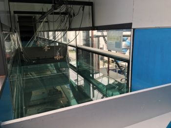
J. Mar. Sci. Eng. 2019, 7, 31 2 of 12
and energy dissipation, highlighting that the main governing design parameter could change depending
on forcing conditions (for short waves the main parameter was the submergence of the barrier, for long
waves it was the width of the chamber). Jalon et al., (2018) [8] presented an analytical model to optimize
the design configuration of a vertical thin barrier concerning different criteria, such as harbor tranquility or
wave energy extraction. Other types of structures, e.g., slotted-, porous-, and Jarlan-type barriers, have also
been widely studied [9,10].
Regarding the experimental studies on vertical semi-submerged barriers, Kriebel et al., (1999) [11]
studied their efficiency under regular and irregular waves in terms of the transmission and reflection
coefficients, while Liu and Al-Banaa, (2004) [2] carried out experiments under solitary waves focusing
on the wave forces acting on the barrier.
Nonetheless, in nature we find swell waves coexisting with wind-driven waves. Swell waves are
described as long-period waves that have been traveling for long distances and in absence of wind
can be locally analyzed by means of standard wave spectra. Wind waves are actively growing due to
forcing action from the local wind, and are characterized as non-regular waves consisting of a spectrum
in continuous evolution. However, most of the experimental studies on wave interaction with maritime
structures such as the ones mentioned, are limited to regular and/or irregular waves generated by
a paddle, without considering (1) the effect of wind forcing on both the incident and reflected swell
wave trains, (2) the interaction of the driven sea waves with the structure and (3) the non-linear
interaction between the different wave field components. Therefore, there is still need for data on
the wave-structure interaction under wind-driven waves superimposed on swell, taking into account
their intrinsic irregular and random complex nature.
The present study is based on a series of laboratory experiments of wave-structure interaction
with paddle-generated regular waves in combination with wind-driven waves, due to wind blowing
in the direction swell propagation. The structure consists of a thin vertical semi-submerged barrier
delimiting a chamber along with an impermeable back wall. This type of structures can be used in
maritime engineering applications such as harbor tranquility and energy extraction [7,8,12].
The manuscript is structured as follows. Section 2 describes the adopted methodology, the experimental
facility and measurements. Section 3 contains the critical analysis of the data and the discussion. Conclusions
are given in Section 4.
2. Methodology
2.1. Experimental Setup and Data Analysis
Experiments were conducted in the Atmosphere-Ocean Interaction Flume (CIAO) of the Andalusian
Institute for Earth System Research, Granada, Spain. It is 16 m long, 1 m wide and is designed for
an optimal water depth of 70 cm (Figure 1). This facility is dedicated to the study of the coupled processes
between the ocean and the atmosphere. It is equipped with (i) two opposite piston-type wavemakers
with active absorption system that allow the generation of regular and irregular waves with periods
between 1–5 s, and therefore in the range of shallow to intermediate conditions, and heights up to
25 cm; (ii) a closed-circuit wind generation system (wind tunnel) with mean wind speed at start of the
test section—representative of U10 conditions in prototype—up to 12 m/s that generate waves with
an effective fetch length up to 12 m, and (iii) a current-generation system for currents of up to 75 cm/s.
The system allows the generation of waves and currents following or opposing the wind direction,
with all the possible combinations. The system allows for the active absorption of incoming waves by
the secondary paddle and the compensation of re-reflection by the generating paddle. More information
on this system and its performance can be found on Lykke Andersen et al., (2016) [13]. For a detailed
description of the CIAO facility the reader is referred to Clavero et al., (2013), Nieto et al., (2015) [14,15].
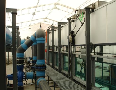
A rigid thin barrier, with a thickness of 1.9 cm and a submergence d was installed vertically (see Figure 2).
This barrier was located at 11 m from the wavemaker and spaced a distance B (width of the chamber) from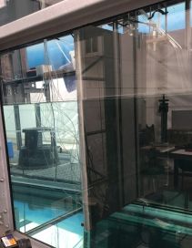
J. Mar. Sci. Eng. 2019, 7, 31                                                                                      3 of 12

a vertical rigid back wall. The x- and z-axes refer to the stream-wise and vertical direction, respectively,
with the origin at the mean water level in the section where the thin barrier is located.

                Figure 1. Atmosphere-Ocean Interaction Flume (CIAO). Schematics provided by VTI.

                                                                       16 m
                                     30 80    42   75        130 cm

                                                                                                          Wind
                                    S7S6     S5 S4S3    S2            S1
                                z                                                                         Paddle
                                                                                                   H, T
                                                   d
                                       B
                                             x                                             11 m

                                                                              S7 S6   S5 S4S3     S2
                                                                  z

                                                                                             d
                                                                                  B
                                                                                       x

      Figure 2. The experimental setup of the flume. The system consists of a semi-submerged rigid thin
      barrier separated a distance B (chamber width) from a vertical rigid back wall. S1–S7 are ultrasound
      distance gauges for free surface elevation measurements. Tests were done with a combination of
      regular waves (paddle-generated) and wind-driven waves traveling in the same direction.

     Water level measurements were obtained using seven UltraLab ULS 80D acoustic wave gauges
installed at different sections along the flume, with a maximum repetition rate equal to 75 Hz, a declared
space resolution of 0.18 mm and a reproducibility of ±0.15%. The overall accuracy is 0.5 mm. Free surface
measurements were taken for 185 s.
     Measurements of wind speed were collected before the installation of the system (vertical plate or
back wall) using a Pitot tube at x = 0 m (plate section) and at different heights above the water level.
The signal was acquired for ≈ 60 s with a data rate of 1 kHz. Figure 3 shows the wind speed profiles
at different rotation rates of the fan used in the tests, with Ure f representing the average speed in
the vertical profile [16].
     A combination of paddle (with H input , T input , representing the r.m.s. wave height and period given
as inputs to wave generation software), and wind waves (Ure f , representing the reference wind speed)
were generated for a chamber with a constant width B = 2.5 m and different plate submergences d.
Each regular wave experiment was performed (i) in the absence of wind, and (ii) in combination with
wind waves using different Ure f . Regular waves were generated using only one of the wavemakers
with the active absorption on.
J. Mar. Sci. Eng. 2019, 7, 31 4 of 12
Uref (m/s)
3.95 5.88 7.88 9.21
0.30
0.25
0.20
z (m)
0.15
0.10
0.05
4 6 8 10
Uw (m/s)
Figure 3. Wind speed profiles (symbols) and reference speed Ure f (dashed vertical lines) for the different
rotation rates of the fan.
Table 1 lists the values of the parameters of the experiments. Hrms0 and Tz0 represent the r.m.s.
wave height and the mean wave period obtained by the statistical analysis of the surface elevation data
in the section of the wave gauge S1 (x = −2.1 m) for the experiment without wind (Ure f = 0 m/s).
The statistical analysis consists on applying the zero-upcrossing technique to the surface elevation
time series obtaining the individual wave heights and periods of the signal. The mean wave
period Tz0 is always coincident with the input period T input , whereas Hrms0 is not coincident with
the imposed value H input . L0 represents the wavelength (experiment without wind) obtained by
means of the linear dispersion equation ω02 = gk0 tanh (k0 h) where ω0 = T2π
z0
is the angular frequency,
k0 = 2π
L0 is the wavenumber and h = 0.7 m is the water depth and Tz0 is the mean wave period
obtained from the experiment without wind. The two first natural oscillation periods of the system
2B
were approximated using Merian’s formula Tn = √ with n = 1, 2, ..., and are equal to T1 = 1.9 s
n gh
and T2 = 0.95 s, respectively. Figure 4 presents the signal of the wave gauge S1 for the different
experiments and different wind conditions.
Table 1. Parameters of the experiments. H input and T input are the input values given to the wave
generation software. Hrms0 , Tz0 and L0 represent the r.m.s. wave height, mean wave period
and wavelength, respectively, obtained by the statistical analysis of the surface elevation data of
S1 for the experiment without wind. The colum Hrms0 depicts the mean value ± the error —when
applicable— between two repetitions of the same case. d/h is the relative submergence, B is the
chamber width and Ure f represents the reference wind speed.
H input Hrms0 T input = Tz0 Ure f
Test d/h B/L0 Tz0 /T1
(cm) (cm) (s) (m/s)
R1a 7 6.4 ± 0.5 1.85 0.33 0.6 0.97 0, 3.95, 5.88, 7.88, 9.21
R1b 7 5 1.85 0.58 0.6 0.97 0, 3.95, 5.88, 7.88, 9.21
R1c 7 8.9 ± 0.15 1.85 0.71 0.6 0.97 0, 3.95, 5.88, 7.88, 9.21
R2a 6 6.3 1.65 0.58 0.7 0.87 0, 3.95, 5.88, 7.88, 9.21
R3a 7 2.7 2.78 0.58 0.4 1.46 0, 3.95, 5.88, 7.88, 9.21
R4a 7 6.7 4.76 0.58 0.2 2.5 0, 3.95, 5.88, 7.88, 9.21
R5a 6 2.8 ± 0.25 3 0.58 0.3 1.58 0, 3.95, 5.88, 7.88, 9.21
R6a 6 5.8 ± 1.4 4.7 0.58 0.2 2.47 0, 3.95, 5.88, 7.88, 9.21J. Mar. Sci. Eng. 2019, 7, 31 5 of 12
Uref (m/s) 0 5.9 9.2
R1a 2.5 R3a
0 0.0
−5 −2.5
5 R1b 5 R4a
0 0
η (cm)
−5
−5
R1c 2.5 R5a
5
0.0
0
−5 −2.5
5 R2a 5 R6a
0 0
−5 −5
0 2 4 6 0 2 4 6
time (s) time (s)
Figure 4. Free surface elevation of the wave gauge S1 for the experiments presented on Table 1. In each
panel, different colors of the lines refer to different wind speeds.
In addition to the statistical analysis by means of the zero-upcrossing technique, data were
processed by spectral analysis using the python Scipy Signal processing functions. The spectra are
obtained with the Welch method, using a Hanning window with 50% overlap resulting in 17 degrees
of freedom and a spectral resolution of 0.039 Hz.
The model investigated in this work can be replicated in real-world applications guaranteeing Froude
similarity, commonly adopted for the design of maritime structures. We notice that using a Froude-based
similarity and working with the same fluid viscosity for both model and prototype, inevitable violates
the Reynolds number scaling. In this case, a partial dynamic √ similarity is achieved using Froude scaling,
with length and pressure scale of λ and a time scale of λ. Assuming a geometrical scale of 1/14,
experiment R1a, e.g., scales to an incident wave height of Hinput = 1 m, Tinput = 7 s, L = 59 m in water
depths of h = 10 m.
2.2. Expected Wave Characteristics
Jalon et al., (2018) [8] presented an analytical model to optimize the design configuration of
a vertical thin barrier concerning different criteria, such as harbor tranquility or wave energy extraction
using a prototype setup as the once presented in this work. Their results showed the presence of
nodal and antinodal frequencies of the spectra on both the leeward and seaward side depending
on the geometrical configuration and the incident wave characteristics focusing on the relative
submergence (d/h) and relative width (B/L) parameters. For values of d/h > 0.25, maximum values
of the reflection coefficient where found for very small values of B/L and slightly larger than 0.5 for
which also maximum capture coefficients were found.
For B/L close to 0.6, the reflection coefficient increases with d/h (experiments R1a-R1c—Table 1)
up to values of d/h ≈ 0.7 when it starts decreasing again. In these cases, the highest capture
coefficient is obtained for d/h ≈ 0.6. At x = 0, their results showed the presence of quasi-nodes
(quasi-antinodes) in the seaward (leeward) sides for the configurations resembling experiments R1a
and R2a and the quasi-antinodes on both sides experiment R1c.
For d/h close to 0.6, and varying B/L (experiments R1b, R3a, R4a) the reflection coefficient
increases with B/L while the transmission coefficient presents similar values for B/L of 0.2 (R4a)
and 0.4 (R3a) and larger values for B/L = 0.6 (R1b). At x = 0, their results showed the presence
of quasi-antinodes (quasi-nodes) in the seaward (leeward) sides for the configurations resembling
experiments R3a and R4a and the opposite for experiment R1b.J. Mar. Sci. Eng. 2019, 7, 31 6 of 12
3. Results and Discussion
The key element of the analysis is the influence of the geometry of the system and of
the wind-generated waves on the measured variables. Therefore, we analyzed the results with
respect to the relative submergence d/h and to the different Ure f . During the experiments, the relative
submergence d/h was modified by varying the submergence of the plate d whereas the water depth h
was kept constant. To test different values of the relative width B/L, the chamber width B remained
fixed and different configurations of wave periods with and without the combination of wind were
tested, changing the wavelength of the incident wave L0 .
All the results presented henceforth are dimensionless with respect to the corresponding values
of the measurements in absence of wind and at Section S1.
Figures 5–8 show the results for the different R1-experiments, corresponding to the same initial
theoretical values H input = 7 cm, T input = 1.85 s and wind speeds, but with a different relative
submergence d/h (see Table 1). The mean wave period of the regular waves (Tz0 = 1.85 s) is very close
to the 1st order natural period of the chamber, with Tz0 /T1 = 0.97.
Figure 5 depicts, in the first and second row, the dimensionless r.m.s. wave height and wavelength
for the gauges S2 (seaward region) and S5, S6 and S7 (leeward region) for each experiment. In the leeward
region, the ratio Hrms /Hrms0 is related to the transmission coefficient. The third row shows the mean
phase lag defined as Φ = ωtmax , with ω being the angular frequency. tmax represents the time difference
of the maximum surface elevation position between the signal of each sensor and the signal of sensor S1
within a wave period. For its calculation, the signal of each sensor is divided into waves of period T input
and the position of the maximum surface elevation is found.
leeward leeward leeward seaward
S7 (x = 1.6 m) S6 (x = 1.3 m) S5 (x = 0.5 m) S2 (x = −0.8 m)
R1a - d/h = 0.33 R1b - d/h = 0.58 R1c - d/h = 0.71
Hrms /Hrms0
2
1
0
1.0
L/L0
0.5
2π
1.5π
1π
Φ
0.5π
0π
0.0 2.5 5.0 7.5 0.0 2.5 5.0 7.5 0.0 2.5 5.0 7.5
Uref (m/s) Uref (m/s) Uref (m/s)
Figure 5. R1a-b-c-experiments with constant input values H input = 7 cm, T input = 1.85 s and different
relative submergences d/h. The first row shows the r.m.s. wave height Hrms , the second row
shows the wavelength L, the third row shows the phase lag Φ. Each panel shows the results for
S5-S6-S7 sensors (violet, green, and blue lines, respectively) in the leeward region, and for sensor
S2 (orange dashed line) in the seaward region. Values are dimensionless with respect to Hrms0 ,
L0 measured in Section S1 without wind.
It can be observed that for each individual sensor and experiment the wave height is constant
regardless of the wind speed, showing that wind-driven waves have almost no influence in
the amplification or reduction of the periodic wave inside the chamber, when Tz0 /T1 ≈ 1. In the case of
the highest plate submergence, d/h = 0.71 (R1c), the minimum value of the wave height is observed.
This result was expected, given the high reflection of the incident wave and the low energy transmitted
inside the chamber. The highest values are obtained for the experiment R1b with d/h = 0.58. In this case,J. Mar. Sci. Eng. 2019, 7, 31 7 of 12
S5 gives a value of Hrms /Hrms0 ≈ 2, showing a resonant behavior inside the chamber. However, a high
variation between the different sensors inside the chamber is observed in this test, with values in the range
0.5–2 between the sensors S7 and S5. It can be attributed to the partial standing pattern inside the chamber
that exhibits a spatial variation of the total wave amplitude with values depending on the relative distance
of each gauge to quasi-nodes and quasi-antinodes. Also, the phase lag shows a similar variability,
with 0.2π < Φ < 0.5π for sensor S5 and 1.5π < Φ < 1.7π for sensor S7. We notice the presence of
quasi-antinodes and surface elevations in phase opposition (Φ ≈ π) which is critical for the study of
the loads acting on the plate [8]. These results are in agreement with the results in Jalon et al., (2019) [8],
where the same structural configuration is studied analytically. The maximum values of the capture
coefficient (a proxy for the transmission coefficient), with the presence of quasi-antinodes, are obtained
for B/L ≈ 0.6 (R1a-b-c-experiments).
The main influence of wind-driven waves is observed in the estimations of L/L0 . As observed,
L/L0 decreases for increasing wind speeds and is more evident for Section S2, where the wind is
expected to have a higher influence. A change of the phase lag can be observed for varying Ure f
for the tests R1a and R1b, whereas for tests R1c, with d/h = 0.71, the phase lag is almost constant;
however, as already highlighted, it varies considerably for different sections. This can be attributed to
the fact that higher reflections are likely to be associated with higher submergences showing partial
standing oscillations. Therefore, a reduction of the non-linear interaction between wind waves and the
periodic component is expected.
Figure 6 depicts the dimensionless surface elevation η/Arms0 , where Arms0 is the r.m.s. wave
amplitude obtained from S1 in the absence of wind. It can be observed that the highest relative
amplitude inside the chamber is given for tests with d/h = 0.33 − 0.58, with almost double of
the seaward wave amplitude at the Section S5 (which is very close to a quasi-antinode), for all
wind speeds. The deformation of the regular wave induced by wind action in the seaward region
is transmitted inside the chamber, where an asymmetry between crests and troughs is observed.
This could be due to the amplification modes of the system and to the re-reflection, both controlled by
geometry. In passing, we notice that free surface oscillations are strongly affected by the forcing term
and by the damping, the latter mainly due to dissipation [17]. For limited dissipation, a blow up of
the oscillations is expected for multiple harmonic in the forcing term. In this respect, the free surface
oscillations in the chamber can vary significantly if energy is extracted.
Uref (m/s) 0 5.9 9.2
leeward seaward
S6 (x = 1.3 m) S5 (x = 0.5 m) S2 (x = −0.8 m)
2.5
0.0 R1a
d/h = 0.33
−2.5
2.5
η/Arms0
0.0 R1b
d/h = 0.58
−2.5
2.5
0.0 R1c
d/h = 0.71
−2.5
0 1 2 3 4 5 60 1 2 3 4 5 6
time (s) time (s)
Figure 6. R1a-b-c-experiments with constant nominal values H input = 7 cm, T input = 1.85 s
and different relative submergences d/h. Free surface elevation is dimensionless with respect to
the amplitude measured at Section S1 in the absence of wind. The left column shows the results for
the two sensors S5–S6 in the leeward region (continuous and dashed lines, respectively), the right
column shows the results for sensor S2 in the seaward region. In each panel, different colors of the lines
refer to different wind speeds.J. Mar. Sci. Eng. 2019, 7, 31 8 of 12
A similar behavior can be observed for all three d/h values tests in Section S2 in the seaward
region, where the wind generates short waves traveling alongside the long regular wave. This effect
is less noticeable in the test with d/h = 0.71 (R1c), where a higher reflection of the periodic wave
components is expected.
These results are mirrored in the power spectrum S0 = S( f ) f p /m0 shown in Figure 7,
dimensionless with respect to the peak frequency f p and to the zeroth-order moment m0 obtained
from data at Section S1 in the absence of wind. At high frequencies, the scenario is controlled
by wind-driven waves, energy increases, and the resonant frequencies become less noticeable.
Inside the chamber the peak frequency in all sections almost corresponds to the frequency of the
regular waves, which is very close to the natural period of the chamber, Tz0 /T1 = 0.97. The energy
is higher for sensor S5 closest to the plate and the energy in the chamber increases with respect to
the seaward region, which is associated with the peak frequency of regular waves and to the first
resonant period, more so for the case with the highest relative submergence d/h = 0.71; there is
an energy decrease at higher frequencies with respect to the seaward side. This is attributed to
non-linear interaction between wind-driven waves, periodic waves and resonant waves controlled by
the geometry of the system and to the filtering effect of the screen, more efficient for high frequency
components. For clear cut results, it will be necessary to further explore the wave profile and its
variation with different geometrical configurations and with different forcing conditions.
Uref (m/s) 0 5.9 9.2
leeward seaward
S6 (x = 1.3 m) S5 (x = 0.5 m) S2 (x = −0.8 m)
10−2 R1a
d/h = 0.33
10−8
10−2 R1b
S0
d/h = 0.58
10−8
10−2 R1c
d/h = 0.71
10−8
100 100
f /fp f /fp
Figure 7. Dimensionless power spectrum S0 . For caption see Figure 6.
Figure 8 shows the dimensionless phase-averaged surface level for the R1a-b-c-experiments,
with and without wind-driven waves and for different sensors. It can be observed that both
the predominant regular wave phase, and the wave profile, change from the seaward to the leeward
region. In the case of the highest relative submergence d/h = 0.71 (R1c), the transmission of the longer
periodic wave is expected to be lower, and the changes could be due to the wind acting on the
free surface. Sensor 5, at section | x |/L = 0.12, shows a wave profile similar to the incident wave,
with an increment in wave height due to its position in a quasi-antinode. Sensor 6 shows a reduction of
the wave height and some changes in wave profile. As expected, due to the shading effect of the plate,
the influence of wind-driven waves is limited to the seaward region, with a more evident variation of
the wave profile for the case of d/h = 0.58 (R1b) and Ure f = 5.9 m/s.
To analyze the effect of the dimensionless parameter B/L in the resonant behavior of the chamber
for different wind conditions, different regular wave (paddle-generated) and wind-wave configurations
were tested for a fixed relative submergence d/h = 0.58. This analysis is especially relevant for the
design of OWC devices that have performance directly related to the oscillation of the water column.J. Mar. Sci. Eng. 2019, 7, 31 9 of 12
Uref (m/s) 0 5.9 9.2
leeward leeward seaward
S6 (x = 1.3 m) S5 (x = 0.5 m) S2 (x = −0.8 m)
R1a
0.0 d/h = 0.33
−2.5
η/Arms0
R1b
0.0 d/h = 0.58
−2.5
R1c
0.0 d/h = 0.71
−2.5
0 0.25 0.5 0.75 1 0 0.25 0.5 0.75 1 0 0.25 0.5 0.75 1
t/Tz0 t/Tz0 t/Tz0
Figure 8. Phase-averaged dimensionless free surface elevations. For caption see Figure 6. The dashed
lines correspond to the phased-averaged value ± one standard deviation.
Figure 9 shows the same variables shown in Figure 5, but the comparison is made between
different regular wave experiments with the same relative submergence d/h = 0.58. Each column
represents two sets of experiments with initial theoretical values of H input = 6–7 cm and similar
values of Tz0 /T1 .
leeward leeward leeward seaward
S7 (x = 1.6 m) S6 (x = 1.3 m) S5 (x = 0.5 m) S2 (x = −0.8 m)
R1b - (7, 1.0) R3a - (7, 1.5) R4a - (7, 2.5)
R2a - (6, 0.9) R5a - (6, 1.6) R6a - (6, 2.5)
6 1.2
2.0
1.0
Hrms /Hrms0
1.5 4
1.0 0.8
2
0.5
0.6
0.0 0
1.0 1.0 1.0
0.8 0.8 0.8
L/L0
0.6 0.6 0.6
0.4 0.4 0.4
0.2 0.2 0.2
2π 2π 2π
1.5π
1.5π 1.5π
1π
Φ
1π 1π
0.5π
0π 0.5π 0.5π
0.0 2.5 5.0 7.5 0.0 2.5 5.0 7.5 0.0 2.5 5.0 7.5
Uref (m/s) Uref (m/s) Uref (m/s)
Figure 9. Experiments with the same relative submergence d/h = 0.58. For caption see Figure 5.
Values of Hrms /Hrms0 ≈ 3 can be observed in the leeward region for tests with Tz0 /T1 ≈ 1.5,
while at Section S2 in the seaward region, results Hrms /Hrms0 ≈ 5 − 6. We notice that the scaling value
of wave height Hrms0 is significantly reduced with respect to the nominal value (Table 1). For example,
R3a was carried out using a nominal wave height of H input = 7 cm while the statistical analysis of S1 for
this experiment without wind gave a value of Hrms0 = 2.7 cm. In this case, at Section S2, the closest toJ. Mar. Sci. Eng. 2019, 7, 31 10 of 12
the plate in the seaward region, very high values of r.m.s. wave height were obtained (higher reflection),
with consequent very high values of Hrms /Hrms0 . It can also be observed that for experiments R4a
and R6a, corresponding to the experiments with higher wave periods of the regular wave, there is
a noticeable stronger influence of wind-driven waves than for experiments with lower wave periods,
characterized by a constant value of Hrms /Hrms0 for the different wind speeds. A reduction of
the wavelength L/L0 can be observed for increasing wind speed for almost all tests. In the seaward
region, there is an almost five-fold reduction with the highest wind. In the leeward region, this influence
changes depending on Tz0 /T1 , e.g., for Tz0 /T1 ≈ 2.5 there is a negligible change of the wavelength
with wind speed.
Another relevant indicator of the system behavior is the phase lag. For tests with Tz0 /T1 ≤ 1.5
the phase lag varies greatly from one sensor to the other for the same experiment, whereas for tests
with Tz0 /T1 ≈ 2.5 results π ≤ Φ ≤ 1.5π regardless of wind speed. Hence, in some tests, the relation
between the period of the incident wave height and the resonant wave periods of the system plays
a major role than the wind speed.
Figure 10 shows Hmax and Hrms of sensors S2, S5, and S6. Each point represents a different
configuration of regular wave (paddle-generated) and wind speed and they were ordered according to
the relation Tz /T1 (x-axis) where Tz is the mean wave period of each sensor and case and T1 the 1st
order natural period of the chamber. The first row presents the results for S2 (seaward region) where
the highest values of H/Hrms0 are achieved. This is due to the fact that as previously explained,
in this position the regular periodic wave component is predominant over the shorter wind waves,
therefore the highest values of wave height are obtained. For the sensors S5-S6 in the leeward region,
an amplification of wave energy is observed for values Tz /T1 close to 1 for all wind speeds. For most
of the experiments in the absence of wind, the same values of Hmax and Hrms are obtained while in
tests with wind, Hmax /Hrms0 presents higher values than Hrms /Hrms0 . This is expected and due to
the fact that the r.m.s. is a statistic that takes into account all the wave heights in the signal, therefore,
taking into account the shorter wind-driven waves, its value is expected to be lower than Hmax .
Uref (m/s) 0 5.9 9.2
Hrms /Hrms0 Hmax /Hrms0
7.5 seaward
S2 (x = −0.8 m)
H/Hrms0
5.0
2.5
0.5 1.0 1.5 2.0 2.5
4
leeward
S5 (x = 0.5 m)
H/Hrms0
2
0
0.50 0.75 1.00 1.25 1.50 1.75 2.00 2.25 2.50
3 leeward
S6 (x = 1.3 m)
H/Hrms0
2
1
0.75 1.00 1.25 1.50 1.75 2.00 2.25 2.50
Tz /T1
Figure 10. Dimensionless maximum and r.m.s. wave heights for different sensors (row-wise). In each
panel, different points correspond to the experiments with the same relative submergence d/h
and different configurations of regular waves (paddle-generated) with and without the combination
of wind waves. In each panel, the different colored lines represent the results for experiments with
and without wind.J. Mar. Sci. Eng. 2019, 7, 31 11 of 12
4. Conclusions
In the present study, the hydrodynamic interaction of regular waves, in combination with short
wind-driven waves, with a vertical fixed semi-submerged barrier was experimentally investigated.
The study was focused on the influence of the seaward wave characteristics and certain geometric
characteristics of the structure, with special attention on the role of wind waves providing new insight
of the influence of wind-driven waves on the incident wave characteristics and in the wave field inside
the chamber as it still remains a topic to be further investigated in maritime and coastal engineering.
A series of conclusions can be derived.
When analyzing a regular wave configuration with a wave period similar to the 1st order natural
period of the chamber, an amplification of wave energy in the seaward region is measured for a relative
submergence of d/h = 0.58, in agreement with the results obtained by Jalon et al., (2019) [8]. In the case
of higher submergences, the fixed plate operates in a highly reflective manner and a reduction of
the wave energy inside the chamber can be observed. Therefore, the submergence of the plate is a key
parameter for the design of these types of structures, either for harbor protection (energy reduction),
or WEC devices (energy amplification).
Wind-driven waves have a high influence on the wave symmetry and phase lag between
the seaward and leeward regions. This is an important factor to take into account since it could
lead to strong forces on the barrier when the phase lag equals π.
The influence of wind waves is more noticeable for the experiments where Tz0 /T1 ≥ 1.5, in which
the short-crested waves proved to have a higher influence on the resulting wave periods and heights in
the seaward region. Therefore, the influence of wind waves on the behavior of the structure depends
greatly on the period of the predominant periodic component (swell).
The overall behavior of the system depends on the relative values of periodic waves, wind waves,
and resonant periods of the chamber. The analysis has been conducted without extracting energy
from the system, since no OWC device was inserted in the experimental layout. In real conditions,
with an OWC device active, we expect some minor modifications, with a general reduction of the wave
height in both leeward and seaward regions. In this respect, the present analysis can be confidently
applied for verifying the structures in the most critical conditions.
As a future extension, this research could involve (i) the analysis of irregular waves, where is
expected that wind waves effects depend on the frequency range; (ii) the analysis of grouping effects,
where a sequence of grouped waves can force the system with presently unnoticed effects.
Author Contributions: All authors conceptualized the study. A.L.-L. did the experimental work and analysis of
data with the guidance of A.B and S.L. All authors contributed to the preparation of the manuscript.
Acknowledgments: A.L.L. is supported by the research group TEP-209 (Junta de Andalucía) and project
AQUACLEW. Project AQUACLEW is part of ERA4CS, an ERA-NET initiated by JPI Climate, and funded
by FORMAS (SE), DLR (DE), BMWFW (AT), IFD (DK), MINECO (ES), ANR (FR) with co-funding by the European
Union (Grant 690462). During the preparation of the manuscript, A.L.L. was doing a research stay at the University
of Parma (PhD cotutelle agreement) funded by the Campus of International Excellence of the Sea (CEIMAR)
and the University of Granada.
Conflicts of Interest: The authors declare no conflict of interest. The funders had no role in the design of the study;
in the collection, analyses, or interpretation of data; in the writing of the manuscript, or in the decision to publish
the results.
References
1. Koutandos, E.; Prinos, P.; Gironella, X. Floating breakwaters under regular and irregular wave forcing:
reflection and transmission characteristics. J. Hydraul. Res. 2005, 43, 174–188. [CrossRef]
2. Liu, P.L.F.; Al-Banaa, K. Solitary wave runup and force on a vertical barrier. J. Fluid Mech. 2004, 505, 225–233.
[CrossRef]
3. Dean, W.R. On the reflexion of surface waves by a submerged plane barrier. Math. Proc. Camb. Philos. Soc.
2008, 41, 231–238. [CrossRef]J. Mar. Sci. Eng. 2019, 7, 31 12 of 12
4. Ursell, F.; Dean, W.R. The effect of a fixed vertical barrier on surface waves in deep water. Math. Proc. Camb.
Philos. Soc. 1947, 43, 374–382. [CrossRef]
5. Losada, I.J.; Losada, M.A.; Roldán, A.J. Propagation of oblique incident waves past rigid vertical thin barriers.
Appl. Ocean Res. 1992, 14, 191–199. [CrossRef]
6. Losada, M.A.; Losada, I.J.; Roldán, A.J. Propagation of oblique incident modulated waves past rigid,
vertical thin barriers. Appl. Ocean Res. 1993, 15, 305–310. [CrossRef]
7. Losada, I.J.; Losada, M.A.; Losada, R. Wave spectrum scattering by vertical thin barriers. Appl. Ocean Res.
1994, 16, 123–128. [CrossRef]
8. Jalón, M.; Lira-Loarca, A.; Baquerizo, A.; Losada, M. An analytical model for oblique wave interaction with
a partially reflective harbor structure. Coast. Eng. 2019, 143, 38–49, doi:10.1016/j.coastaleng.2018.10.015.
[CrossRef]
9. Bennett, G.S.; McIver, P.; Smallman, J.V. A mathematical model of a slotted wavescreen breakwater.
Coast. Eng. 1992, 18, 231–249. [CrossRef]
10. Isaacson, M.; Premasiri, S.; Yang, G. Wave interactions with vertical slotted barrier. J. Waterw. Port Coast.
Ocean Eng. 1998, 124, 118–126. [CrossRef]
11. Kriebel, D.; Sollitt, C.; Gerken, W. Wave forces on a vertical wave barrier. In Proceedings of the 26th
International Conference on Coastal Engineering, Copenhagen, Denmark, 22–26 June 1998; pp. 2069–2081.
12. Karimirad, M. Offshore Energy Structures; Springer International Publishing: Cham, Switzerland, 2014; p. 298.
13. Lykke Andersen, T.; Clavero, M.; Frigaard, P.; Losada, M.; Puyol, J. A new active absorption system and its
performance to linear and non-linear waves. Coast. Eng. 2016, 114, 47–60. doi:10.1016/j.coastaleng.2016.04.010.
[CrossRef]
14. Clavero, M.; Aguilera, L.; Nieto, S.; Longo, S.; Losada, M.A. Experimental study of the interaction
atmosphere-ocean. In Proceedings of the XII Coast and Ports Spanish Conference, Cartagena, Spain,
7–8 May 2013.
15. Nieto, S.; Lira-Loarca, A.; Clavero, M.; Losada, M.A. Canal de Interacción Atmósfera-Océano (CIAO).
In Proceedings of the XIII Coast and Ports Spanish Conference, Avilés (Asturias), Spain, 24–25 June 2015.
16. Addona, F. Swell and Wind-Waves Interaction under Partial Reflection Conditions. Ph.D. Thesis,
University of Parma, Parma, Italy and University of Granada, Granada, Spain, 2018.
17. Longo, S.; Chiapponi, L.; Liang, D. Analytical study of the water surface fluctuations induced by
grid-stirred turbulence. Appl. Math. Model. 2013, 37, 7206–7222. [CrossRef]
c 2019 by the authors. Licensee MDPI, Basel, Switzerland. This article is an open access
article distributed under the terms and conditions of the Creative Commons Attribution
(CC BY) license (http://creativecommons.org/licenses/by/4.0/).You can also read