Reliability and lifetime of LEDs - Application Note
←
→
Page content transcription
If your browser does not render page correctly, please read the page content below
www.osram-os.com

Application Note No. AN006

Reliability and lifetime of LEDs

Application Note
                                                    Valid for:
                                                    Infrared Emitters; visible LEDs

Abstract
This application note provides a fundamental insight into the topics of “reliability” and
“lifetime”. The terms lifetime and reliability are explained in further detail with respect to light
emitting diodes (LEDs) and how these terms are understood by OSRAM Opto
Semiconductors. In addition, important factors which influence the lifetime and reliability of
LEDs are described. The appendix provides descriptions of the mathematical foundations
that are needed in practice.

                                                                  Author: Lutz Thomas / Ritzer Markus

2020-02-26 | Document No.: AN006                                                              1 / 18
www.osram-os.com
Table of contents
A. Introduction .............................................................................................................2
B. The concept of reliability at OSRAM Opto Semiconductors ..................................2
C. Reliability of LEDs ...................................................................................................3
Extrinsic reliability period ....................................................................................4
Intrinsic reliability period .....................................................................................5
D. Validation and confirmation of reliability and lifetime ...........................................11
E. On-site support regarding reliability and lifetime ..................................................13
F. Appendix ...............................................................................................................13
Fundamentals — definition of terms .................................................................13
Failure rate ........................................................................................................14
Distributions for reliability analysis ....................................................................16
A. Introduction
With the increasing complexity of technical equipment, modules or even
individual components, the aspects of reliability and lifetime and thus the costs
involved with exchange and revision become increasingly more important for the
customer. Here, one must consider an optimization between requirements,
functions and costs over the lifetime of the product.
The single requirement that the device will not fail is no longer sufficient for
modern, powerful components or devices. More often, it is additionally expected
that they perform their required functions without failure. However, it is only
possible to make a prognosis (probability) supported by statistics and
experiments as to what extent such requirements can be fulfilled. A direct
answer or statement as to whether an individual device or component will
operate without failure for a certain period of time cannot be given.
Nowadays, modern methods of quality management and reliability modeling are
used in order to investigate and verify these types of questions.
B. The concept of reliability at OSRAM Opto Semiconductors
Zero Tolerance to Defects (ZTTD) is a rigid part of the corporate culture at
OSRAM Opto Semiconductors. Only in this way is it possible for our customers
to also aim for zero defects in their production and applications.
2020-02-26 | Document No.: AN006 2 / 18www.osram-os.com
OSRAM Opto Semiconductors associates the term reliability with the fulfillment
of customer expectations over the expected lifetime. In other words, the LED
does not fail during its lifetime under the given environmental and functional
conditions. The reliability of the products is thus based on the chain of the
materials, the manufacturing process and the function of the component
(Figure 1). In addition, the final application must also be taken into consideration.
High reliability can only be achieved if the changing effects and
interdependencies of the individual components are already taken into account
during the development phase.
Neglecting this entirely or only focusing on one or two elements leads to a
reduction in the quality of the product and thus, to a decrease in reliability.
Figure 1: Basis of reliability of LEDs
Material
Function
Process
C. Reliability of LEDs
The reliability of a semiconductor element is the property that states how reliable
a function assigned to the product is fulfilled within a period of time. It is subject
to a stochastic process and is described by the probability of survival R(t).
A fault or failure is indicated if the component can no longer fulfill the functionality
assigned to it.
Failures and failure rates are subdivided into three phases:
1. Early failures
2. Random or spontaneous failures
3. Wear-out period
2020-02-26 | Document No.: AN006 3 / 18www.osram-os.com
Since the failure rate is especially high at the beginning and end of the product
cycle, the failure rate over time takes the form of a “bathtub” curve (Figure 2).
Thereby each single failure mechanism exhibits its own chronological
progression and shows therefore an individual bath-tub curve.
For each of these phases, many different types of definitions, analysis methods
and mathematical formulas for reliability can be found in the literature. The most
important definitions and methods which apply to LEDs are described in this
section and in the appendix.
Figure 2: Failure rate over time (“bathtube curve”)
Failure rate
1: Early failure period
2: Spontanous failure period
3: Wear-out period
1. 2. 3.
Time
For the sake of simplicity, the first two phases are combined into a so-called
“extrinsic reliability period”. The third phase, the wear-out period, is
correspondingly designated as the “intrinsic reliability period”.
Extrinsic reliability period
Extrinsic failures (early and spontaneous failures) are generated by defective
materials, deviations in the manufacturing process. More than 99 % of these
extrinsic failures can be observed during installation of the parts in the
application (e.g. by soldering) or in the first hours of operation. In contrast,
between the early failure period and the wearout period, the spontaneous failure
rate for LEDs is extremely low.
In reliability mathematics, this failure period is described by an exponential
distribution. An exponential distribution is based on a constant failure rate over
time. The average failure rate is given in FIT (Failure unITs).
As a rule, an experimental determination of the middle failure rate is extremely
difficult. For this reason, OSRAM Opto Semiconductors uses the SN 29500
standard from Siemens AG, which incorporates the experience of failures in the
field into the typical failure rates for LEDs (Figure 3). In the process, no distinction
is made in regard to the cause of the individual failures.
2020-02-26 | Document No.: AN006 4 / 18www.osram-os.com
Figure 3: LED failure rate in the extrinsic period according to Siemens Standard
SN29500
12
Random failure rate λ [FIT]
SN 29500-12 (2008)
10 for large power packages
8
6
4
2
0
0 2000 4000 6000 8000 10000
Time [h]
Intrinsic reliability period
The intrinsic reliability period describes the so-called wear-out period of the
component at the end of the product cycle. It is based on increased wear and
aging of the material. This continuous change over time is generally measurable
and is referred to as degradation. For LEDs, the most significant degradation
parameters are the changes in brightness or color coordinates. Other
parameters play a subordinate role.
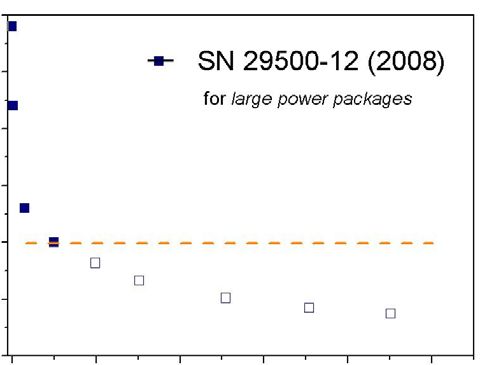
During operation, LEDs experience a gradual decrease in luminous flux,
measured in Lumens. As a rule, this is accelerated by the operating current and
temperature of the LED and also appears when the LED is driven within
specifications (Figure 4).
The term “Lumen maintenance” (L) is used in connection with the degradation of
light in LEDs. This describes the remaining luminous flux over time, with respect
to the original luminous flux of the LED.
Due to continuous degradation, a failure criterion must be established in order to
obtain a concrete evaluation of the LED failure. The point in time at which the
luminous flux of the LED reaches the failure criterion is then described as the
lifetime of the LED.
As a rule, the failure criterion is determined by the application. Typical values are
50 % (L50) or 70 % (L70), depending on the market of the LED product.
2020-02-26 | Document No.: AN006 5 / 18www.osram-os.com
Figure 4: Degradation curve
100
Relative light output [%] 90
80
70
L70
60 100
00
50
40
30
20
10
0
1 10 100 1,000 10,000 100,000
Time [h]
Since aging is based on a change in the material properties and is therefore
subject to statistical processes, the lifetime values also are based on a statistical
distribution.
The percentage of components that have failed is described by the term
“mortality” (B). A value of B50 thus describes the point in time at which 50 % of
the components have failed. This value is generally specified as typical median
lifetime, t50 or tml, for LEDs. In addition to the median value (B50), a value can
also be specified when 10 % of the components have failed (B10 value). This
allows one to draw a conclusion about the width of the lifetime distribution
(Figure 5).
2020-02-26 | Document No.: AN006 6 / 18www.osram-os.com
Figure 5: Cumulative failure distribution showing the lifetime
99 %
Cumulated failure distribution
90 %
50 %
B50
16 %
10 %
B10
1%
0.1 %
100 ppm
10 ppm
1 ppm
t10 t50
1 10 100 1,000 10,000 100,000
Time [h]
However, for thermo-mechanical stress on a component (e.g. temperature
cycles), the continuous aging process generally cannot be measured. This
means that the constant aging process that leads to failure cannot be described
by means of a characteristic measurement parameter such as light degradation
during electrical operation. An extrapolation of the degradation curve to a
defined failure criterion as is shown in Figure 4 is not possible, here. In this case,
in order to be able to make statements about the time of failure or the failure
distribution, tests must be carried out until the first abrupt failures occur. An
example of this is fatigue in adhesive or bonded connections.Influencing factors
with respect to reliability and lifetime
Similar to conventional lights, the reliability and lifetime of LED light sources are
also dependent on various factors, or can be influenced by these factors. The
most important physical influencing factors include humidity, temperature,
current and voltage, mechanical forces, chemicals and light radiation (Figure 6).
2020-02-26 | Document No.: AN006 7 / 18www.osram-os.com
Figure 6: Influencing factors on reliability and lifetime
Humidity
Temperature
Chemicals
LED Reliability
Light
Mechanical forces
Current and voltage
These can even lead, in a worst case situation, to a total failure or influence the
aging characteristics in the long term (e.g. brightness), and thus produce a
change in the reliability and lifetime. Such direct influencing factors are the
temperature and resulting junction temperature Tj(unction) of the LED, for
example, but the amount of current used to drive the LED is also an influencing
factor. Under otherwise equal operating conditions, an increase in the ambient
temperature as well as an increase in current produces an increase in the
junction temperature. In general, however, an increase in junction temperature
brings about a decrease in lifetime (Figure 7).
Figure 7: Dependence of lifetime on the junction temperature and solder point
temperature
OSLON® Black LY H9GP
110,000
100,000
90,000
Lifetime B10/L70 [h]
80,000
70,000
TS TJ
60,000
50,000
40,000
30,000
20,000
IF = 1000 mA / L70/B10
10,000
0
0 20 40 60 80 100 120 140 160
Temperature [°C]
2020-02-26 | Document No.: AN006 8 / 18www.osram-os.com
Another direct influencing factor is mechanical force. If large mechanical forces
are applied to the LED, for example, this generally results in damage which can
additionally lead to total failure of the LED. The origin of the individual factors can
be found in different areas such as LED design, LED processing, the customer
application and the environment and from there, can be traced back to various
aspects and parameters (Figure 8). If these four areas are examined in more
detail, it can be determined that three of the four areas can be directly influenced
by the LED manufacturer or the user. The last area, the environment, ultimately
cannot be changed and must be considered as a given in the application.
For example, the source of the influencing factor, temperature, can be assigned
to two areas: LED design and the customer application. In the area of LED
design, the source of the temperature influence lies both with the electrical
parameters and with the transfer of heat.
Figure 8: Sources of influencing factors
LED design Customer application
• electrical parameters • heat transport
• heat transport • PCB layout and material
• ESD layout ESD protection
• package • electrical circuit
Reliability
Assembly Envirnonment
• storage condition • ambient temperature
• soldering process • temperature cycles
• handling (pick & place; • humidity
ESD) • pollution
• light radiation
Depending on the current applied (IF) and the associated voltage (UF), a power
dissipation is created, which to a large extent, is converted into heat. This leads
to an increase in temperature in the junction of the LED. The amount of power
dissipation is proportional to changes in the junction temperature.
The proportionality factor is the thermal resistance of the housing
(Rth, Junction-Solderpoint) of the LED. This reflects the heat transfer characteristics
of the LED.
The lower the thermal resistance of the LED, the better the thermal properties of
the LED become. If heat is transfered efficiently out of the package, the junction
temperature increase is not as high. As an example, two components with
differing Rth values (2.5 and 8 K/W) are examined at the same solder point
temperature TS = 100 °C and the same operating conditions (current) (Figure 9).
The junction temperature of the component with low thermal resistance only
increases to ~ 115 °C. In contrast, however, the component with the higher
thermal resistance exhibits a junction temperature of > 144 °C. As mentioned
2020-02-26 | Document No.: AN006 9 / 18www.osram-os.com
previously, the lifetime of an LED is reduced with an increase in the junction
temperature. At the same solder point temperature, the component with the
lower Rth achieves a longer lifetime than the component with the higher Rth. In
addition to an increased lifetime, lower thermal resistance offers an additional
advantage: At the same solder temperature, a component with a low Rth
achieves a higher light output. The reason for this is the decrease in efficiency of
an LED with an increase in junction temperature. For the LED manufacturer, the
influencing factors that have a significant influence on lifetime and reliability can
already be taken into consideration in the development phase.
Figure 9: The dependency of lifetime on temperature due to the influence of various Rth
values (example)
110,000
Ts Ts TJ/TJ
100,000
90,000 'TJ-S
80,000
Lifetime [h]
70,000
60,000
50,000 'TJ-S
40,000
30,000
Low Rth High Rth
20,000
Ts TJ Ts TJ
10,000
IF = 1000mA / L70/B10
0
0 20 40 60 80 100 120 140 160
Temperature [°C]
The impacts of these factors can be reduced through the following measures:
• Robust design
• Optimal thermal management
• Stable and optimized production processes in order to minimize the risk of
spontaneous failure
• Customer support for including LED designs in the customer application
In the area of customer applications, the influencing factor of temperature can
be traced back to heat dissipation. Here, the layout and material of the printed
circuit board (PCB) play an important role.
Summarized under the term “thermal management” which among other things,
includes the selection of an appropriate PCB material (e.g. FR4, IMS), the layout
of LEDs, the component density, additional cooling, etc., the user also has the
2020-02-26 | Document No.: AN006 10 / 18www.osram-os.com
opportunity to specifically target his application to accommodate for the
influencing factors.
The following measures can be taken:
• Optimal thermal board management
• Optimal design for efficient use of the LED
• Handling the LED according to specifications
• Considering the strengths and weaknesses of LEDs
An insufficient thermal management directly leads to a reduction of the reliability
and lifetime of the LED. For more information and an exact description on how
the thermal resistance is determined for the individual packaging types at
OSRAM Opto Semiconductors please refer to the application note “Package-
related thermal resistance of LEDs”.
However, in general it can be ascertained, that in spite of the high reliability of
OSRAM Opto Semiconductors LEDs, only through the consideration of all areas
and all changing effects and dependencies a high overall or system reliability can
be achieved.
D. Validation and confirmation of reliability and lifetime
All LED packages and chip families from OSRAM Opto Semiconductors undergo
a number of tests for validation and confirmation of reliability and lifetime. The
selection of tests, test conditions and duration occurs by means of an internal
OSRAM Opto Semiconductors qualification specification based on JEDEC, MIL
and IEC standards. In addition, the requirements profile of the component is also
included.
The following Table 1 shows the list of typically performed tests. In addition, the
various test conditions, the test duration and the stress factors involved are
listed.
Based on the internal OSRAM Opto Semiconductors qualification specification
and the requirements profile, the selection of the test, the test conditions and test
duration can be set.
The mechanical stability of an LED is checked by means of a solder heat
resistance test as well as powered and unpowered temperature cycle tests.
Here, the cycle count and the temperature difference serve as measures of
stability. These types of tests are also drawn upon to evaluate the failure rate.
For proof of reliability, the LEDs undergo individual tests of up to 1000 hours in
duration. If the properties and interactions of the integral parts of the LED are
known, results can be taken from already tested products and applied to other
types of LEDs with the same material characteristics. As a result, the general test
scope is reduced, since fewer products must be tested. This allows the test
duration of individual products to be increased to a longer period.
2020-02-26 | Document No.: AN006 11 / 18www.osram-os.com
At OSRAM Opto Semiconductors, tests sequences are carried out for up to
10,000 hours, for example, in order to investigate general effects. Individual
technology platforms are even evaluated for more than 35,000 hours.
Table 1: Example reliability test matrix for OSRAM Opto Semiconductors LEDs
Test Conditions Duration Stress factors
Resistance to Solder Reflow 3 runs Temperature,
Heat (RSH) Soldering Chemicals,
JESD22-A113 260 °C / 10 sec Mechanical forces
Resistance to Solder Wave soldering 3 runs Temperature,
Heat, Through the Wave 260 °C / sec Chemicals,
(RSH-TTW) Mechanical forces
JESD22-B106
Wet High Temperature T = 85 °C 1000 h Temperature,
Operating Life (WHTOL) R.H. = 85 % Humidity
JESD22-A101 IF = 5 mA / 10 mA
Temperature Cycle (TC) - 40 °C / + 125 °C 1000 cycles Mechanical forces
JESD22-A104 15 min at extreme
temperatures
Power Temp. Cycling - 40 / + 85 °C 1000 h Temperature,
(PTC) IF = [max. derating] Current,
JESD22-A105 ton/off = 5 min Mechanical forces
High Temperature T = 25 °C 1000 h Temperature,
Operating Life (HTOL) IF = [max. derating] Current
JESD22-A108
High Temperature T = 85 °C 1000 h Temperature,
Operating Life (HTOL) IF = [max. derating] Current
JESD22-A108
Pulsed life test (PLT) T = 25 °C 1000 h Temperature,
JESD22-A108 IF = [max. derating] Current
ESD-HBM Human body model 1 pulse per Voltage
ANSI/ESDA/JEDEC JS- 2000 V polarity
001-2010 lt. AEC Q102 direction
These types of selective, extremely long-term investigations provide a solid
basis for calculation of the lifetime. According to OSRAM Opto Semiconductors,
however, the resulting test data should not be “blindly” extrapolated to
determine the average lifetime. Rather, this data should make it possible to
understand why the different materials used behave the way they do.
This allows a highly reliable extrapolation or prediction of the product
performance characteristics to be made, which is confirmed by a small deviation
from target values.
2020-02-26 | Document No.: AN006 12 / 18www.osram-os.com
Statements about lifetime that are based on mathematical results without test
data and background knowledge should generally be viewed with caution.
E. On-site support regarding reliability and lifetime
OSRAM Opto Semiconductors supports its customers worldwide. This already
begins in the pre-sales phase. OSRAM Opto Semiconductors offers its
customers assistance with the selection of an appropriate light source and
advises them in implementing an optimally executed application. In addition, we
support you with our technical expertise regarding quality and reliability.
For further information and questions regarding the lifetime and reliability of
particular LED products, our corresponding sales representatives and/or
subsidiaries are available to offer assistance.
F. Appendix
Fundamentals — definition of terms
In the following, the most important and relevant terms and definitions from the
areas of quality management and statistics are presented, as well as an example
for a reliability distribution.
Reliability and failure probability. Reliability R(t) states the probability P, that a
system or individual component remains functional during a time-frame t under
normal operating and environmental conditions. In complementary terms, one
speaks of the probability of failure F(t) or unreliability.
Thus, if n components are driven under the same conditions and the number of
failures is r(t) at time t, then the following applies:
rt
F t = ------- = 1 – R t
n
At the beginning, all components function properly (time t = 0) and at some point,
they all are defective. That is,
R t = 0 = 1 and R t = 0
This means that the probability of failure F(t) of a component starts at 0 (0 %) and
increases to 1 (100 %) over time — an inverse relation to reliability.
Probability of failure density (failure density). The failure density f(t) states the
probability of a failure at a time t, with respect to a time interval dt.
Mathematically, it represents the derivation of the probability of failure.
dF t PT t dR t
f t = ------------ = -------------------- = – ------------
dt dt dt
2020-02-26 | Document No.: AN006 13 / 18www.osram-os.com
Figure 10: Relation between reliability R(t) and probability of failure F(T)
1 F(t)
Probability
0.5
R(t)
0
t
Failure rate
The failure rate λ(t) is an important indicator for the reliability of lifetime of an
object. It describes the probability of a failure within a time interval dt, with
respect to the components that are functional at time t.
ft ft
t = --------- = -----------------
R t 1 – Ft
The failure rate states how many units fail on average within a period of time.
Usually, failure rates are given in units of [1/time unit] such as 1 failure per hour
(-1/h).
Due to the low failure rate of electronic components, this is often stated as a FIT:
1 failure
FIT = ---------------------------------------------------
9
10 component hours
Component hours = number of components * hours of operation
In general, the failure rate is not constant. In many cases, the failure rate usually
follows the so-called “bathtub curve” over the entire component life cycle
(Figure 11). The chronological sequence is comprised of three phases.
2020-02-26 | Document No.: AN006 14 / 18www.osram-os.com
Figure 11: Chronological progression of failure rate
Failure rate
λ(t)
Economic life
Early failure due to
Increase due to
weaknesses in the material,
aging, wearout, fatigue,
quality fluctations, application Random etc.
failures failure
Early failure period Spontanous failure period Wearout period
Phase I — the early failure period. At the beginning of the product lifetime, a
higher failure rate can be observed, which quickly falls off over time. This phase
can be described with a Weibull distribution. This is generally caused by design
defects, weakness in the material, quality fluctuations in production or through
application failures (dimensioning, handling, testing, operation, etc.) or unreal,
unconfirmed failures.
Phase II — with constant failure rate. This phase corresponds to the actual
period of economic usefulness. In this phase, the failure rate is constant and can
be described with an exponential or Poisson distribution. Here, failures mostly
appear suddenly and purely at random.
Phase III — wearout failures. In this phase, the failure rate increases at a faster
rate due to aging, wearout, fatigue, etc. with continuous operation. This phase
also can be described by a Weibull distribution.
With the representation and interpretation of bathtub curves, it should generally
be kept in mind that in most cases, the curve is only based on a few test points.
The mathematical description is therefore somewhat imprecise, due to
deviations and test-related scattering. A reliable representation is therefore only
possible if a statistically large quantity of data has been obtained.
In practice, it can also happen that the time periods of the individual phases are
significantly different. Depending on the complexity of the object and the
maturity of the manufacturing process, the initial failure period may not be
present at all or may be characterized by a period of up to a few thousand hours
of operation.
In order to minimize the failure rate, specific preventative measures are already
carried out by OSRAM Opto Semiconductors during the development phase as
well as in the subsequent manufacturing phase. In addition, the failure rate is
strongly influenced by the predominant operating conditions. For example, for
2020-02-26 | Document No.: AN006 15 / 18www.osram-os.com
classic semiconductor elements, the failure rate doubles when the junction
temperature increases by 10 to 20 °C.
Distributions for reliability analysis
The Weibull and exponential distribution functions used for describing the
bathtub curve are described in more detail in the following.
Weibull distribution. Due to its flexibility, the Weibull distribution is well suited
to statistical analysis of all types (areas I to III of the bathtub curve). The primary
advantage of this function is that the curve can be adjusted with the shape
parameter b. In this way, a large number of well established fixed-form
distributions (such as normal, log, exponential distributions, etc.) can be realized
(Figure 12).
Figure 12: Weibull distribution for various shape parameters b and with a characteristic
lifetime of T = 1
Failure density f(t)
Failure rate λ(t)
lifetime t lifetime t
Failure probability F(t)
Reliability R(t)
lifetime t lifetime t
With a shape parameter b < 1, a decreasing failure rate (area I) is described, with
b = 1, a constant failure rate (area II — exponential distribution) is described and
with b > 1, an increasing failure rate (area III) is described.
In the biparametric form of the Weibull distribution, the probability of failure F(t)
and its complement, reliability R(t), become:
b
– --
t
T
Ft = 1 – e ,b>0
t b
– --
T
Rt = e ,b>0
2020-02-26 | Document No.: AN006 16 / 18www.osram-os.com
Their density function f(t) and failure λ(t) result in:
b
– --
t
b t b–1 T
f t = --- -- e , b>0
T T
b–1
t = --- --
b t
, b>0
T T
, where b = shape factor and T = characteristic lifetime.
Exponential distribution. The exponential distribution particularly represents
the lifetime distribution in Phase II of the bathtub curve, the area of random
failures. The failure rate is assumed to be constant over time.
With the exponential distribution, the following applies:
Probability of failure:
– t
Ft = 1 – e , t 0 and > 0
Reliability:
– t
Rt = e , t 0 and > 0
Failure rate:
1 1
t = = -- = --------------
T MTTF
In this area and in connection with irreparable systems, the term MTTF (mean
time to failure) is used to describe to average lifetime.
For a lifetime distribution with a constant failure rate, this means that at the
MTTF, the probability of failure is around 63 % or that on average, approximately
2/3 of all components have failed.
– t 1
Ft = 1 – e ,where t = MTTF and = --------------
MTTF
– -------------- MTTF
1
MTTF
F MTTF = 1 – e
–1 1
F MTTF = 1 – e = 1 – --
e
F MTTF = 63.2 %
2020-02-26 | Document No.: AN006 17 / 18www.osram-os.com
Don't forget: LED Light for you is your place to
be whenever you are looking for information or
worldwide partners for your LED Lighting
project.
www.ledlightforyou.com
ABOUT OSRAM OPTO SEMICONDUCTORS
OSRAM, Munich, Germany is one of the two leading light manufacturers in the world. Its subsidiary, OSRAM
Opto Semiconductors GmbH in Regensburg (Germany), offers its customers solutions based on semiconduc-
tor technology for lighting, sensor and visualization applications. OSRAM Opto Semiconductors has produc-
tion sites in Regensburg (Germany), Penang (Malaysia) and Wuxi (China). Its headquarters for North America
is in Sunnyvale (USA), and for Asia in Hong Kong. OSRAM Opto Semiconductors also has sales offices th-
roughout the world. For more information go to www.osram-os.com.
DISCLAIMER
PLEASE CAREFULLY READ THE BELOW TERMS AND CONDITIONS BEFORE USING THE INFORMA-
TION SHOWN HEREIN. IF YOU DO NOT AGREE WITH ANY OF THESE TERMS AND CONDITIONS, DO
NOT USE THE INFORMATION.
The information provided in this general information document was formulated using the utmost care; howe-
ver, it is provided by OSRAM Opto Semiconductors GmbH on an “as is” basis. Thus, OSRAM Opto Semicon-
ductors GmbH does not expressly or implicitly assume any warranty or liability whatsoever in relation to this
information, including – but not limited to – warranties for correctness, completeness, marketability, fitness
for any specific purpose, title, or non-infringement of rights. In no event shall OSRAM Opto Semiconductors
GmbH be liable – regardless of the legal theory – for any direct, indirect, special, incidental, exemplary, con-
sequential, or punitive damages arising from the use of this information. This limitation shall apply even if
OSRAM Opto Semiconductors GmbH has been advised of possible damages. As some jurisdictions do not
allow the exclusion of certain warranties or limitations of liabilities, the above limitations and exclusions might
not apply. In such cases, the liability of OSRAM Opto Semiconductors GmbH is limited to the greatest extent
permitted in law.
OSRAM Opto Semiconductors GmbH may change the provided information at any time without giving notice
to users and is not obliged to provide any maintenance or support related to the provided information. The
provided information is based on special conditions, which means that the possibility of changes cannot be
precluded.
Any rights not expressly granted herein are reserved. Other than the right to use the information provided in
this document, no other rights are granted nor shall any obligations requiring the granting of further rights be
inferred. Any and all rights and licenses regarding patents and patent applications are expressly excluded.
It is prohibited to reproduce, transfer, distribute, or store all or part of the content of this document in any form
without the prior written permission of OSRAM Opto Semiconductors GmbH unless required to do so in ac-
cordance with applicable law.
OSRAM Opto Semiconductors GmbH
Head office:
Leibnizstr. 4
93055 Regensburg
Germany
www.osram-os.com
2020-02-26 | Document No.: AN006 18 / 18You can also read