Supplementary Materials for - Partisan pandemic: How partisanship and public health concerns affect individuals' social mobility during COVID-19 ...

advances.sciencemag.org/cgi/content/full/sciadv.abd7204/DC1

 Supplementary Materials for

Partisan pandemic: How partisanship and public health concerns affect individuals’
 social mobility during COVID-19
 J. Clinton*, J. Cohen, J. Lapinski and M. Trussler

 *Corresponding author. Email: josh.clinton@vanderbilt.edu

 Published 11 December 2020, Sci. Adv. 6, eabd7204 (2020)
 DOI: 10.1126/sciadv.abd7204

This PDF file includes:

 Materials and Methods
 Figs. S1 to S18
 Tables S1 to S3

Materials and Methods
Section S1: Study design materials and methods
All the data and code needed to replicate the study is available in Dryad at:
https://doi.org/10.5061/dryad.3bk3j9khg
To obtain our data, we interview of 1,135,638 randomly selected respondents from the Survey
Monkey platform between April 4, 2020 and September 29, 2020. These individuals are
randomly sampled from the approximately 2 million individuals who take Survey Monkey
surveys every day.
The data we analyze was collected by Survey Monkey using respondents who have consented to
participate in the Survey Monkey audience panel and surveys.
The privacy policy that Survey Monkey respondents agree to is available at:
https://www.surveymonkey.com/mp/legal/privacy-policy/
The privacy policy pertaining to survey research that respondents consent to when participating
in Survey Monkey is available at:
https://www.surveymonkey.com/mp/legal/survey-research-privacy-notice/
The policy governing the content of Survey Monkey surveys is available at:
https://www.surveymonkey.com/mp/legal/content-policy/
The survey was written and administered by Survey Monkey and provided to the other
collaborators on this project. Because the surveys were designed, administered, and collected by
Survey Monkey and provided to the researchers, IRB approval was not required. In addition,
because the survey data being provided to the researchers is anonymous and includes only non-
sensitive data, the project would be IRB exempt even had the collaborators designed the survey
questions being analyzed.
The anonymized data are weighted for age, race, sex, education, and geography using the Census
Bureau’s American Community Survey to reflect the demographic composition of the United
States. An additional smoothing parameter for political party identification based on aggregates
of SurveyMonkey research surveys is included. Weights are generated each day using daily
interviews Monday through Friday, and once over combined interviews on Saturday and Sunday.
Party identification parameters are refreshed bi-weekly.
Figure S1 Displays the number of valid responses to our key dependent variable on each day
from April 4th to September 29, 2020.
The following question is asked to determine an individual’s degree of social activity, which
serves as our main dependent variable.
In the past 24 hours, have you left your home to do any of the following? (Select all that apply)
[Response order randomized]
 • Go to work
 • Go grocery shopping

 1

• Exercise
 • Go for a walk/get some fresh air
 • Visit with friends of family
 • Eat at a restaurant of bar
 • Get medical care
 • None of the above
To measure each individual’s level of activity in the previous 24-hours, we add up the number of
activities they reported participating in. We are cognizant of the fact that this combines activities
that are voluntary (like going to a restaurant) and those that are involuntary (like getting medical
care). Figure S2 displays the trends in each of these activities over our time, and clearly there is
much more variation in more voluntary activities. To probe these differences, in Figure S4 and
S5 below we report the partisan differences in each of these activities. While there is notable
heterogeneity, in each activity the same pattern of partisan-motivated activity is present.

The following question was asked to gauge an individual’s level of worried about COVID-19:

How worried are you that you or someone in your family will be exposed to the coronavirus?
 • Very worried
 • Somewhat worried
 • Not too worried
 • Not worried at all
To classify individuals as partisans they are asked the following questions:
In politics today, do you consider yourself a Republican, Democrat, or Independent?
 • Republican
 • Democrat
 • Independent
[If respondent selects “Independent”] As of today, do you lean more to the Republican or
Democratic Party?
 • Republican
 • Democrat
 • Neither
If respondent answers Republican or Democrat in the first question, or leans towards either of
those parties in the second question, they are classified accordingly. Respondents who select
“Neither” on the second question are classified as “independent”.

 2

We also include two media questions to help determine whether partisan values are activated by
media consumption.
To determine overall media diet we ask:
How much do you keep up with the news, regardless of whether you get it from television,
newspapers, radio, or any other source?
 • A lot
 • Some
 • Not Much
 • Not Much at all
Individuals who answer “A lot” are coded as High News Consumers, and those that any
otherwise are coded as non-High News Consumers.
To determine the proportion of an individual’s media diet that is made up of right-wing news
sources we ask the following question:

Do you follow political news coverage by any of the following media organizations on a daily or
almost daily basis?

 • Breitbart
 • Buzzfeed
 • CNN
 • Drudge Report
 • FOX News
 • MSNBC
 • New York Times
 • NPR
 • Washington Post
 • Wall Street Journal
 • None of the above

Individuals are given a right-wing media score by dividing the number of right-wing media
sources they report following (FOX News and Breitbart) by the total number of media sources
they report following. As such, the maximum of this score is 1, and the minimum 0.
Data on COVID-19 prevalence comes from COVID-19 Data Repository by the Center for
Systems Science and Engineering (CSSE) at Johns Hopkins University. These data report, on
each day, the number of COVID-19 cases in each county in the United States.
As a first data processing step, we use county population estimates from the American
Community Survey to transform county cases to be cases per 1000 residents.
We then calculate for each county, for each week, the change in the number of cases from the
previous week in that county, using the median number of cases in each county for each week.
 3

Consider, for example, interviewing an individual in zip-code 37206 (in Davidson county on
Nashville’s East Side) on April 4th. On the week of April 4th in Davidson county (in which the
zip-code is wholly contained) the median number of cases per 1000 was 1.001. In the week
previous, the median number of cases per 1000 was .428. This individual, therefore, would be
given the value .573 for change in county cases per 1000. This value is a fair representation of
the fact that this individual, on this day, was witnessing a worsening public health situation in
their immediate surrounding.
Survey Monkey respondents self-report their zip-code. To assign respondents to a county we
determine the county in which the majority of the residents of that zip-code live in. For 86% of
respondents, their zip-code is entirely contained within one county.
Finally, we merge the data on how the number of COVID-19 cases is changing in each county on
each day to the Survey Monkey data.
Section S2. Method of Statistical Analysis
Our methodology estimates the following 4 models separately on each day t for individuals i in
states j.
 Equation 1
 24' = + + ' + '+
 Equation 2
 24' = + + γ ' + ' + + '+
 Equation 3
 24' = + + . ℎ . . . ' + ' + +
 Equation 4
 24' = + + ' + ' + . ℎ . . . '
 + ' + '+

On each day, we regress the level of self-reported activity in the last 24 hours for individual i in
state j on state fixed-effects (αj) (to control for between-state differences ) and a matrix of
individual-level and zip-code level demographics (Ki). These demographics are gender (dummy
for female), age (dummies for 18-24, 25-34, 34-44, 45-54, 55-64, 65+), race (dummies for
White, Black, Asian, Hispanic, and other), education (dummies for less than high school, high
school only, associates or some college, bachelor degree, postgraduate degree) , income (
dummies for below 29.9k, 30k-74.9k, 75k-149.9k, +150k ), zip code population density
(dummies for urban, suburban, and rural), and employment status (dummy for unemployed).
In all models, standard errors are clustered at the state level.
To estimate the coefficients of partial determination for Figure 2, we calculate the following
equation using specifications 1, 2, & 3:
 K|M = ( PQRK|M − PQRT )/ PQRT
Thus, the quantity K|M is the proportion of unexplained variance in specification 1 that is
explained by adding partisanship (in specification 2) or public health (in specification 3).

 4

To obtain standard errors for these estimates we perform a bootstrapping procedure. On each day
we randomly sample (with replacement) rows from the dataset to construct a bootstrap sample
the same length as the day’s original sample. In this bootstrap sample we estimate specifications
1-3 and record the coefficients of partial determination. We complete this procedure 1000 times
per day. The standard errors in Figure 2 represent the 95% distribution of these bootstrap
estimates.
Figure 3 represents the daily coefficients on the two-party variables and change in county cases
on each day from specification (4). The 95% confidence intervals are derived from the standard
errors from the OLS model, which are clustered by state.
The coefficients in Figure 4 come from regressions using specification (4) run separately in each
state. For these regressions, individuals are pooled across days, so a polynomial time trend is
employed. The values on the x axis are, for each state, the aggressiveness of their COVID-19
mitigation policy. The details of this measure can be found below in section S6.

Section S3. Robustness of Results: Using Specific Activity Measures instead of Sum Total
Our main dependent variable is an additive index of activities the respondent has participated in
over the previous 24-hours. This scale includes both voluntary and involuntary activities. A
reasonable critique is that partisanship’s effects on this measure is being driven entirely by
differential activity in voluntary activity.
To investigate this, we repeat our main analysis separately for each activity.
Figure S4 presents results from specification (4) run separately on each activity, pooled across
time with a polynomial time trend. While there are important differences, in each activity
partisanship is a significant differentiator for activity. As with the main results in the paper, these
results cannot be explained by differences between states (as the models include state fixed
effects), nor can they be explained by an individual’s age, race, income, education,
unemployment status, or population density of their community.
Figure S5 presents results from running specification (4) on each activity on each day, to
determine the trends in the impact of partisanship. Interestingly, some activities (like going to
work or walking) have seen persistent partisan differences across time. Others seem to be far
more affected by time.

Section S4. Robustness of Results: Differences in Leaners and Identified Partisans

In Table S1 we present a pooled model using specification (4) where party “leaners” are
separated. As mentioned in the main text, political science literature has consistently found that
leaners behave in ways broadly similar to identified partisans. The results in this case support
that conclusion. Democrat leaners and identified Democrats are similarly less likely to be
socially active compared to Independents, and Republican leaners and identified Republicans are
similarly more likely to be socially active compared to Independents. Indeed, in the case of
levels of activity during this pandemic, being a leaner is more impactful than being an identified
partisan. Table S2 presents a more restrictive model with Zip-Code fixed effects – which does

 5

even more to control for the statutory environment an individual is living in. The results are
unchanged: party has a robust effect on social behavior.

Section S5. Robustness of Results: Alternative Measures of COVID-19 Impact

For our main analyses we used as a measure of public health the weekly change in the number of
cases per 1000 in a respondent’s county. We believe that this is a reasonable measure of how an
individual’s immediate public health situation is changing. However, to show the robustness of
our findings in this section we replicate Figure 2 in the paper using various other measures of
public health: the weekly change in the number of deaths in an individual’s county, the total
number of cases in an individual’s county, the total number of deaths in an individual’s county,
the weekly change in the number of cases in an individual’s state, and the weekly change in the
number of deaths in an individual’s state. Note that for these last two measures we drop the state
fixed effects from the specification, as otherwise the model would not be able to be estimated.
All specifications show identical results to those found in the paper.

There is slightly more evidence of an effect of COVID-19 using the statewide measure. It may
be that statewide numbers are more apparent to an individual through news reports then COVID
incidence in their counties. We further investigate this possibility in Table S3, which re-runs
specifications 1-4 using state change in COVID-19 cases in the previous week per 1000 state
residents. Indeed, in this specification, the marginal effect on this variable is slightly higher. The
coefficient of partial determination for change in state cases/1000 is .26, meaning that .26% of
the residual variation in specification 1 is explained by the changing level of COVID-19 at the
state level. This is slightly higher than .22% of variance explained by change in county
cases/1000. Regardless, this state-level measure is still swamped by party. Overall, the two party
variables explain 23 times more variation than the state-level measure of COVID-19 change.

An additional note is that it is impossible to determine whether a larger relationship between
COVID incidence and social mobility at the state level is due to individuals reactions to the
incidence of COVID in their community, or to statewide regulations. That is, individuals may be
less mobile in states with a higher incidence of COVID simply because that state has taken more
aggressive steps to limit mobility.

S6: Robustness in Results: Trends in Partisan Effects by State

Our main estimates of the impact of partisanship use state fixed-effects to rule out the
relationships being driven by statutory regulations in different states. That is, these fixed-effects
rule out democrats being less socially mobile because more democrats live in states which have
more restrictive COVID mitigation laws. This being said, it may still be the case that the
relationship between partisanship and distancing might be driven by the partisans in certain
states, while other states have no differences.

Figure 4 in the main body of the paper displays the results of a pooled model between
partisanship and distancing in each state, showing that there is a remarkably similar effect of
being a partisan on distancing in every state. Figure S15 extends this analysis, graphing the
average number of activities practiced by Democrats and Republicans on each day and in each
state. Again, this figure shows a remarkable degree of similarity in partisan behavior across the

 6

country. In every state, the average Republican participates in more activities than the average
Democrat throughout the time series. Nearly every state follows the same pattern as well: with
Republicans rapidly increasing their activity levels in April and May, before cutting down on
activity through the summer. Recent months has seen Republicans in nearly every state begin to
increase their activity levels again, however.

S7: Robustness of Results: Varying Relationships Based on Media Consumption

A key finding from Figure 4 in the main text is that the effect of party does not vary a great deal
from state-to-state. That is, Republicans are more socially active (and Democrats less) than
independents at approximately the same rate regardless of state. One explanation for this
uniformity is an increasingly nationalized communication environment (31,33), whereby all
individuals in the country consume an ever greater share of national over local news. Instead of
receiving news about local conditions, high news consumers are likely to receive a national
partisan message about how Democrats and Republicans are expected to behave.

A testable implication of the theory that national partisan messaging is driving these trends is
that the relationship between party and social activity should be stronger for individuals who
consume more news. For 82930 individuals from May 27th to June 8th, and an additional 32568
individuals from September 21th to September 29th, Survey Monkey asked respondents: "How
much do you keep up with the news, regardless of whether you get it from television,
newspapers, radio, or any other source?". We coded those who answered “A lot” as high news
consumers (1), and those who answered “Some”, “Not Much”, and “Not at all” non-high news
consumers (0). To understand the degree to which watching the news changes the impact of
partisanship, we interact this variable with the indicators for Democrat, Republican, and Case
Change in our pooled model (i.e. Table S1). The results of this model can be found in Figure
S16. These results confirm the hypothesis: individuals who are high news consumers have a
significantly higher association between their partisanship and social activity than those
individuals who are not high news consumers. Our belief is that this is due to those individuals
being more likely to receive partisan cues about behavior. Being a high news consumer, on the
other hand, does not affect the impact of the number of cases in an individual’s immediate area
on social activities. While the amount of news significantly moderates the effect of party on
distancing behavior, it should be noted that news consumption does not fully explain the effect.
Low news Republicans are still massively more socially mobile than low news Democrats.

A subset of this question is whether specific types of media sources which push a particular type
of message influence an individual’s behavior. Consistent with the President’s stated strategy,
right-wing news sources have consistently downplayed the virus. An important research question
is whether this messaging is associated with decreased concern about COVID-19 among
Republicans. For 5811 individuals from March 9th to March 13th, and an additional 24822
respondents from September 21st to September 29th Survey Monkey asked whether they viewed
several prominent media sources on a “daily or almost daily basis”.1 From these data we create a
variable that measures the proportion of their media diet which consists of two right wing
sources – FOX News and Breitbart. For example: if an individual reported reading 6 news

1
 The full list of sources asked about is: Breitbart, Buzzfeed, CNN, Drudge Report, FOX News, MSNBC, New York
Times, NPR, Washington Post, and the Wall Street Journal.

 7

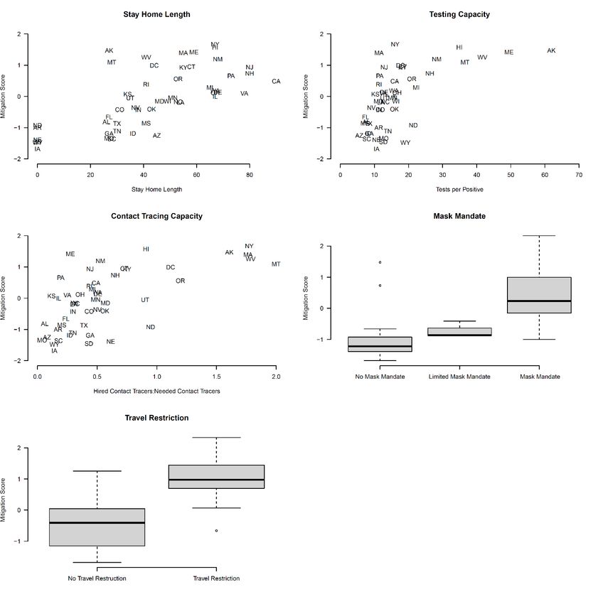
sources, and two of those were Breitbart and FOX News, they would receive a score of .33. The
median Republican has a score of 0.5 of this variable. A full 40% of Republicans score 1 on this
measure, indicating that their only reported news sources are right-wing news sources.

This right-wing media variable was then interacted with the party and case change variables. The
result of this model can be found in Figure S17.

The results confirm the expectation that viewing right wing media sources is associated with less
concern for COVID-19 among Republicans. Republicans who do not watch these news sources
are predicted to be 23 percentage points less worried about COVID-19 than independents.
Republicans whose entire reported media diet consist of right-wing news sources, on the other
hand, are 30 percentage points less worried about COVID-19 than independents. While this
change in marginal effects is significant, it is also important to note that media viewership does
not fully explain the difference between Democrats and Republicans. Even Republicans who
completely abstain from FOX and Breitbart are far less concerned about the virus than are
Democrats or Independents.

S8: Measuring Variation in Social Mitigation by State

Figure 4 in the main text requires the creation of a state-by-state measure of the policy response
to COVID-19. To do so we collected data on several indicators of policy. All data was collected
on August 13th, 2020.

 (1) The length of the states’ stay-at-home order, measured in days. California’s stay at home
 order was (as of this writing) never rescinded. As such it was coded as being 10 days
 longer than the next longest SAH order (a total of 90 days).
 (2) Whether the state had no mask order (0), a limited mask order (for example, only for
 essential workers) (1), or a broad mask order (2).
 (3) Whether the state put any restriction on travel (1) or not (0), such as quarantines for
 visitors from COVID-19 hotspots.
 (4) The proportion of total COVID-19 tests for every positive case, to measure testing
 capacity.
 (5) The proportion of contact tracers hired to contact tracers needed (excluding reserve
 capacity), to measure contact tracing capacity.

Data on stay at home length, mask orders, and travel restrictions was collected from the National
Academy for State Health Policy.2 Testing data was collected from The COVID Tracking
Project.3 Data on contact tracing capacity and need was collected from NPR.4

Because each of these measures are on a different scale, the first data processing step was
standardizing the variables by mean centering each and dividing by the standard error. To scale

2
 https://www.nashp.org/governors-prioritize-health-for-all/
3
 https://covidtracking.com/data/download
4
 https://www.npr.org/sections/health-shots/2020/06/18/879787448/as-states-reopen-do-they-have-the-workforce-
they-need-to-stop-coronavirus-outbre

 8

the measures together we used Principal Component Analysis5 with 1 factor. Factor loadings
ranged from .62 for mask orders to .69 for travel restrictions. This tight band of loadings gives
confidence that each of these underlying components is an important part of robust policy
response. Figure S18 displays how each of the underlying components relates to the recovered
measure of policy mitigation.

5
 Specifically, we used the principal() command from the “psych” package in R.

 9

Figure S1: Daily Number of Respondents to “Last 24-hr activity measure.” The number of responses fluctuates
daily due to the differences in the number of respondents who were invite to participate each day because of
demands for other surveys as well as in the timing of when respondents choose to respond to a request to take a
survey. A total of 1,135,668 responses were analyzed.

 10

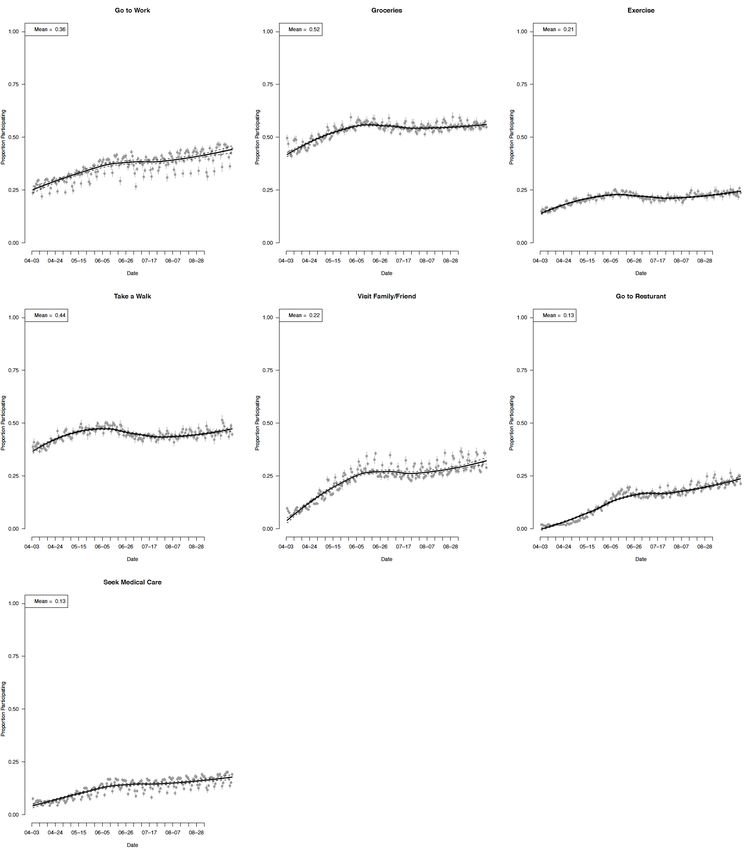
Figure S2: Overall Daily Trends in each Social Activity used to create the “Last 24hr activity” measure. Each
response was weighted equally to create the measure analyzed in the text. Lines characterize the smoothed trend.
While there are differences in the level of activity by activity the trend change similalry over time. Daily estimates
are weighted to US adult population.

 11

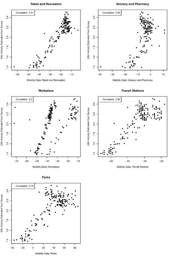
Figure S3: Comparison of Statewide Average of Total Self-Reported Activity to Google Mobility Data. To
validate the survey-based measures of social mobility we analyze, figure plots the average number of total social
activities by state pooled over time (y-axis, weighted by US adult population) against Google’s mobility measure for
various geographic locations (x-axis). The Google mobility data was obtained: October 12, 2020. Our survey
measure of mobility correlates strongly to this behavioral measure.

 12

Figure S4. Coefficient plot of Specification (4) by Social Activity. Results predict the probability of
engaging in each of the social activities by partisanship and COVID-19 incidence to show robustness of
partisan differences across activities. Each row graphs the coefficient estimates from a separate pooled
regression that includes a polynomial time trend, state fixed effects, and a battery of demographics. For
party variables, reference is pure independents. Standard errors are clustered by state. Estimated weighted
by US adult population. There are large and statistically significant partisan gaps in behavior for
behaviors of all types. Further, the incidence of COVID in an individuals area negatively influences the
degree of social mobility, though to a much smaller degree.

 13

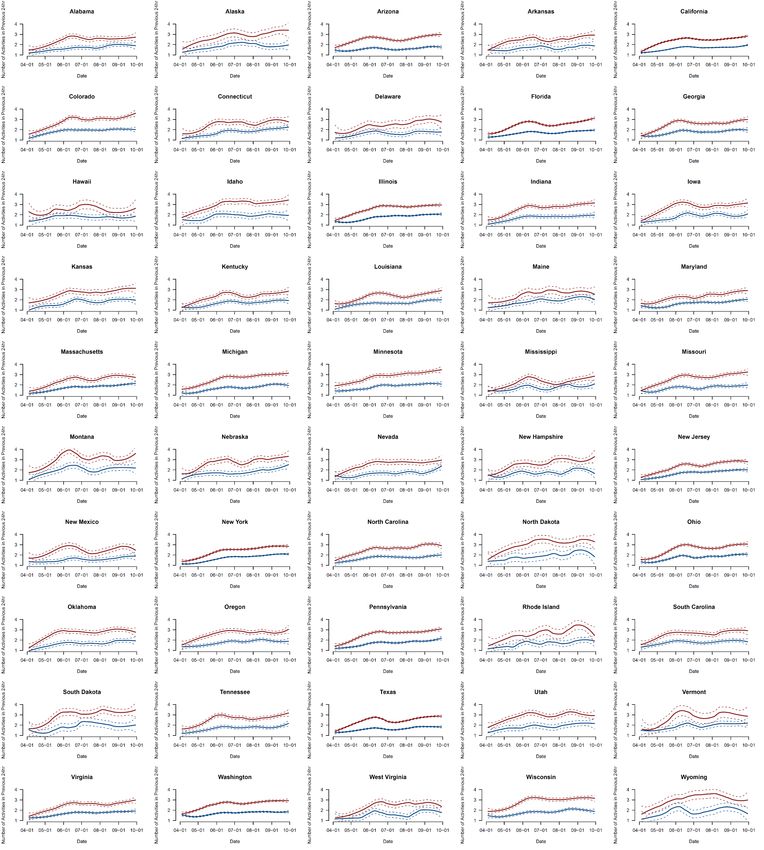
Figure S5: Effect of Partisanship and COVID-19 on Individual Activities Over Time. Coefficients
are from OLS regression using specification (4) run separately on each day. Observations weighted to the
US adult population. For party variables, reference is pure independents. Partisan leaners are included
with identifying partisans. 95% confidence intervals from OLS standard errors clustered by state. Trend is
local regression weighted by inverse of each estimates standard error.

 14

Fig. S6. Variation in Social Mobility Behavior Explained by Partisanship and the Impact of
COVID-19 in the Community (Change in County Deaths/1000). The daily coefficients of partial
determinations are computed via OLS regression using specifications (1-3) run separately on each day.
Observations weighted to the US adult population. Point estimates describe the percent of residual
variation in specification (1) using the weighted national responses for each day being explained by each
variable. The smoothed trend-line is a local regression fitted to the estimates over time. Variation in
changes in the population adjusted COVID-19 reported death rate in the county do not explain variation
in self-reported social mobility.

 15

Fig. S7. Variation in Social Mobility Behavior Explained by Partisanship and the Impact of
COVID-19 in the Community (County Cases/1000). The daily coefficients of partial determinations
are computed via OLS regression using specifications (1-3) run separately on each day. Observations
weighted to the US adult population. Point estimates describe the percent of residual variation in
specification (1) using the weighted national responses for each day being explained by each variable.
The smoothed trend-line is a local regression fitted to the estimates over time. Variation in in the
population adjusted COVID-19 reported number of cases in the county do not explain variation in self-
reported social mobility.

 16

Fig. S8. Variation in Social Mobility Behavior Explained by Partisanship and the Impact of
COVID-19 in the Community (County Deaths/1000). The daily coefficients of partial determinations
are computed via OLS regression using specifications (1-3) run separately on each day. Observations
weighted to the US adult population. Point estimates describe the percent of residual variation in
specification (1) using the weighted national responses for each day being explained by each variable.
The smoothed trend-line is a local regression fitted to the estimates over time. Variation in in the
population adjusted COVID-19 reported number of deaths in the county do not explain variation in self-
reported social mobility.

 17

Fig. S9. Variation in Social Mobility Behavior Explained by Partisanship and the Impact of
COVID-19 in the Community (Change in State Cases/1000). The daily coefficients of partial
determinations are computed via OLS regression using specifications (1-3) run separately on each day.
Observations weighted to the US adult population. Point estimates describe the percent of residual
variation in specification (1) using the weighted national responses for each day being explained by each
variable. The smoothed trend-line is a local regression fitted to the estimates over time. Variation in in
the population adjusted COVID-19 reported change in the number of cases in the state do not explain
variation in self-reported social mobility.

 18

Fig. S10. Variation in Social Mobility Behavior Explained by Partisanship and the Impact of
COVID-19 in the Community (Change in State Deaths/1000). The daily coefficients of partial
determinations are computed via OLS regression using specifications (1-3) run separately on each day.
Observations weighted to the US adult population. Point estimates describe the percent of residual
variation in specification (1) using the weighted national responses for each day being explained by each
variable. The smoothed trend-line is a local regression fitted to the estimates over time. Variation in in
the population adjusted COVID-19 reported change in the number of deaths in the state do not explain
variation in self-reported social mobility.

 19

Fig. S11. Variation in Social Mobility Behavior Explained by Partisanship and the Impact of
COVID-19 in the Community (State Cases/1000). The daily coefficients of partial determinations are
computed via OLS regression using specifications (1-3) run separately on each day. Observations
weighted to the US adult population. Point estimates describe the percent of residual variation in
specification (1) using the weighted national responses for each day being explained by each variable.
The smoothed trend-line is a local regression fitted to the estimates over time. Variation in in the
population adjusted COVID-19 reported number of cases in the state do not explain variation in self-
reported social mobility.

 20

Fig. S12. Variation in Social Mobility Behavior Explained by Partisanship and the Impact of
COVID-19 in the Community (State Deaths/1000). The daily coefficients of partial determinations are
computed via OLS regression using specifications (1-3) run separately on each day. Observations
weighted to the US adult population. Point estimates describe the percent of residual variation in
specification (1) using the weighted national responses for each day being explained by each variable.
The smoothed trend-line is a local regression fitted to the estimates over time. Variation in in the
population adjusted COVID-19 reported the number of deaths in the state do not explain variation in self-
reported social mobility.

 21

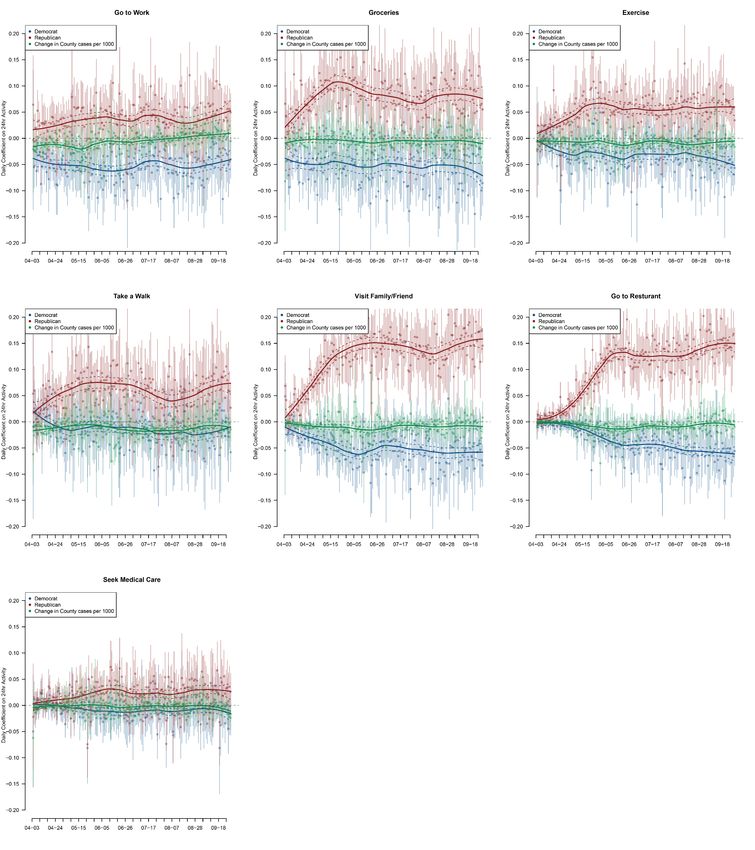
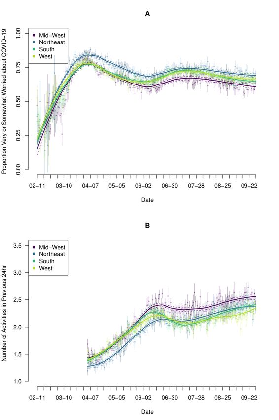
Fig. S13. Concern with Catching COVID-19 and Social Mobility Behavior Over time by Age Group. Plot (A)
graphs the nationally weighted daily percentage of respondents who are either “very” or “somewhat” worried about
catching COVID-19 by age group. Plot (B) graphs the average number of social activities individuals report doing
in the last 24 hours by age group. 95% confidence intervals are reported for each daily average. Estimates weighted
to US adult population. Plotted lines are loess smoothers to summarize trends over time.

 22

Fig. S14. Concern with Catching COVID-19 and Social Mobility Behavior Over time by Census Region. Plot
(A) graphs the nationally weighted daily percentage of respondents who are “very” or “somewhat” worried about
catching COVID-19 by region. Plot (B) graphs the average number of social activities individuals report doing in
the last 24 hours by region. Estimates weighted to US adult population. 95% confidence intervals are reported for
each daily average. Plotted lines are loess smoothers to summarize trends over time.

 23

Fig. S15. Trends in Social Mobility for Democrats and Republicans, by State. Each plot graphs the weighted (to
state adult population) daily average of the number of social activities individuals reported doing in the last 24
hours. For readability, the point estimates for the daily averages are omitted and a loess smoothed curve is used to
show trends over time.

 24

Fig. S16. Effects of Party and Case Change, by News Viewership. Marginal effects from a model predicting
number of social activities performed in last 24 hours. Model is pooled across time and includes a polynomial
time trend, state fixed effects, and a battery of demographics. Estimates weighted by US adult population.
Standard errors are clustered by state. High news consumption significantly increases the effect of party
for both Democrats and Republicans, but does not impact the effect of a change in local cases. However,
even low news Republicans and Democrats are still extremely different in their behavior.

 25

Fig. S17. Effects of Party by Right Wing News Viewership. Marginal effects from a model predicting probability
respondents is worried about COVID-19. Model is pooled across time and includes a polynomial time trend,
state fixed effects, and a battery of demographics. Estimates weighted to US adult population. Standard
errors are clustered by state. Having a media diet with a higher proportion of right wing news (FOX News
and Breitbart) is associated with Republicans being less concerned about COVID. While this change in
concern is statistically significant, it is not of high substantial importance: Republicans who watch no
right-wing media are still far less worried about COVID then Democrats who watch a great deal of these
sources.

 26

Fig. S18. Relationship of Underlying Measures to Mitigation Score. To summarize the extent to which there was
variation in the severity of the regulations used to try to control the spread of COIVD-19, we factor analyze the
various policy decisions being made by each state to uncover a single factor that summarizes the between-state
variation. To do so we standardize each variable and then use a Principal Components Analysis to recover the
dominant factor we use to examine the effect of variation in mitigation policies on variation in social mobility.

 27

Determinants of Social Distancing Behavior

 Last 24 Hour Activity (0-7)

 Time 0.01*
 (0.0005)
 Time2 -0.0000*
 (0.0000)
 Democrat -0.27*
 (0.01)
 Lean Democrat -0.28*
 (0.01)
 Lean Republican 0.54*
 (0.01)
 Republican 0.50*
 (0.01)
 County Change in Covid Cases/1000 -0.08*
 (0.01)
 Female -0.34*
 (0.01)
 Income 30k-74K 0.09*
 (0.01)
 Income 75k-149k 0.20*
 (0.01)
 Income 150k+ 0.31*
 (0.01)
 Age 25-34 -0.09*
 (0.01)
 Age 34-44 -0.14*
 (0.01)
 Age 45-54 -0.19*
 (0.02)
 Age 55-64 -0.26*
 (0.02)
 Age 65+ -0.31*
 (0.02)
 Race Other 0.10*
 (0.01)
 Black 0.04*
 (0.01)
 Asian -0.34*
 (0.02)
 Hispanic -0.06*
 (0.02)
 High School 0.06*
 (0.02)
 Associates/Some College 0.15*
 (0.02)
 College 0.16*
 (0.02)
 Postgraduate 0.13*
 (0.02)
 Unemployed -0.40*
 (0.01)
 Rural 0.03*
 (0.01)
 Urban -0.04*
 (0.01)
 State F.E. Yes
 N 1034346
 Adj. R-squared 0.15
 Residual Std. Error 1.47 (df = 1034268)

 *** p < [.***]; **p < [.**]; *p < .05

Table S1. Number of Social Activities Regression Results with Leaners. Specification analyzes data pooled over time to allow social mobility to vary between
“leaners” and “partisans.” The similarity of coefficients reveals the lack of difference and the justification for collapsing. Standard errors are clustered by state. Data
weighted to US adult population.

 28

Determinants of Social Distancing Behavior

 Last 24 Hour Activity (0-7)

 Time 0.01*
 (0.0001)
 Time2 -0.0000*
 (0.0000)
 Democrat -0.26*
 (0.005)
 Lean Democrat -0.29*
 (0.01)
 Lean Republican 0.54*
 (0.01)
 Republican 0.50*
 (0.01)
 County Change in Covid Cases/1000 -0.08*
 (0.002)
 Female -0.34*
 (0.003)
 Income 30k-74K 0.08*
 (0.005)
 Income 75k-149k 0.19*
 (0.01)
 Income 150k+ 0.29*
 (0.01)
 Age 25-34 -0.08*
 (0.01)
 Age 34-44 -0.13*
 (0.01)
 Age 45-54 -0.18*
 (0.01)
 Age 55-64 -0.26*
 (0.01)
 Age 65+ -0.32*
 (0.01)
 Race Other 0.13*
 (0.01)
 Black 0.10*
 (0.01)
 Asian -0.29*
 (0.01)
 Hispanic -0.004
 (0.01)
 High School 0.05*
 (0.01)
 Associates/Some College 0.14*
 (0.01)
 College 0.15*
 (0.01)
 Postgraduate 0.11*
 (0.01)
 Unemployed -0.40*
 (0.004)
 Zip Code F.E. Yes
 N 1034870
 Adj. R-squared 0.16
 Residual Std. Error 1.47 (df = 1006725)
 ***
 p < [.***]; **p < [.**]; *p < .05
Table S2. Number of Social Activities Regression Results with Leaners (Zip Code FE). Specification analyzes data pooled over time to allow social mobility to
vary between “leaners” and “partisans.” The similarity of coefficients reveals the lack of difference and the justification for collapsing. Standard errors are clustered
by Zip-Code. Data weighted to US adult population.

 29

Determinants of Social Distancing Behavior

 Last 24 Hour Activity (0-7)
 Model 1 Model 2 Model 3 Model 4

 Time 0.01* 0.01* 0.02* 0.01*
 (0.001) (0.001) (0.001) (0.001)
 Time2 -0.0000* -0.0000* -0.0001* -0.0001*
 (0.0000) (0.0000) (0.0000) (0.0000)
 Democrat -0.27* -0.27*
 (0.01) (0.01)
 Republican 0.51* 0.51*
 (0.01) (0.01)
 State Change in Covid Cases/1000 -0.12* -0.12*
 (0.02) (0.02)
 Female -0.43* -0.34* -0.43* -0.34*
 (0.01) (0.01) (0.01) (0.01)
 Income 30k-74K 0.11* 0.09* 0.11* 0.09*
 (0.01) (0.01) (0.01) (0.01)
 Income 75k-149k 0.25* 0.20* 0.25* 0.20*
 (0.01) (0.01) (0.01) (0.01)
 Income 150k+ 0.38* 0.31* 0.38* 0.31*
 (0.02) (0.01) (0.02) (0.01)
 Age 25-34 -0.06* -0.09* -0.06* -0.09*
 (0.01) (0.01) (0.01) (0.01)
 Age 34-44 -0.08* -0.13* -0.08* -0.14*
 (0.01) (0.01) (0.01) (0.01)
 Age 45-54 -0.10* -0.18* -0.10* -0.18*
 (0.02) (0.02) (0.02) (0.02)
 Age 55-64 -0.17* -0.26* -0.17* -0.26*
 (0.02) (0.02) (0.02) (0.02)
 Age 65+ -0.24* -0.31* -0.25* -0.31*
 (0.02) (0.02) (0.02) (0.02)
 Race Other 0.07* 0.10* 0.07* 0.10*
 (0.02) (0.01) (0.02) (0.01)
 Black -0.20* 0.04* -0.20* 0.04*
 (0.02) (0.01) (0.02) (0.01)
 Asian -0.40* -0.34* -0.39* -0.34*
 (0.02) (0.02) (0.02) (0.02)
 Hispanic -0.17* -0.08* -0.17* -0.08*
 (0.03) (0.02) (0.03) (0.02)
 High School 0.07* 0.06* 0.07* 0.06*
 (0.02) (0.02) (0.02) (0.02)
 Associates/Some College 0.14* 0.15* 0.14* 0.15*
 (0.02) (0.02) (0.02) (0.02)
 College 0.09* 0.16* 0.09* 0.16*
 (0.02) (0.02) (0.02) (0.02)
 Postgraduate -0.01 0.13* -0.01 0.13*
 (0.02) (0.02) (0.02) (0.02)
 Unemployed -0.43* -0.40* -0.42* -0.40*
 (0.01) (0.01) (0.01) (0.01)
 Rural 0.09* 0.04* 0.09* 0.04*
 (0.01) (0.01) (0.01) (0.01)
 Urban -0.11* -0.05* -0.11* -0.05*
 (0.01) (0.01) (0.01) (0.01)
 State F.E. Yes
 N 1049411 1034373 1049411 1034373
 Adj. R-squared 0.10 0.15 0.11 0.15
 Residual Std. Error 1.51 (df = 1049338) 1.47 (df = 1034298) 1.51 (df = 1049337) 1.47 (df = 1034297)
 ***
 p < [.***]; **p < [.**]; *p < .05

Table S3. Number of Social Activities Regression Results, State-Wide COVID-19 Measure. Specification analyzes data pooled over time to determine the impact
of the change in the number of COVID-19 cases at the state level. COVID-19 cases measured at the state level are slightly more predictive of distancing than the
equivalent measure at the county level, though still far less important than partisanship. Standard errors are clustered by State. Data weighted to US adult population.

 30