Computational Image Marking on Metals via Laser Induced Heating
←
→
Page content transcription
If your browser does not render page correctly, please read the page content below

Computational Image Marking on Metals via Laser Induced Heating
SEBASTIAN CUCERCA, Max Planck Institute for Informatics, Germany
PIOTR DIDYK, Università della Svizzera italiana, Switzerland
HANS-PETER SEIDEL, Max Planck Institute for Informatics, Germany
VAHID BABAEI, Max Planck Institute for Informatics, Germany

Fig. 1. Laser marked images on stainless steel using our proposed method (the plates are 13 × 13 cm). Images © Piotr Didyk, Alexandr Ivanov, Sebastian
Cucerca.

Laser irradiation induces colors on some industrially important materials,                   ACM Reference format:
such as stainless steel and titanium. It is however challenging to find marking              Sebastian Cucerca, Piotr Didyk, Hans-Peter Seidel, and Vahid Babaei. 2020.
configurations that create colorful, high-resolution images. The brute-force                 Computational Image Marking on Metals via Laser Induced Heating. ACM
solution to the gamut exploration problem does not scale with the high-                      Trans. Graph. 39, 4, Article 1 (July 2020), 12 pages.
dimensional design space of laser marking. Moreover, there exists no color                   https://doi.org/10.1145/3386569.3392423
reproduction workflow capable of reproducing color images with laser mark-
ing. Here, we propose a measurement-based, data-driven performance space
                                                                                             1   INTRODUCTION
exploration of the color laser marking process. We formulate this exploration
as a search for the Pareto optimal solutions to a multi-objective optimization               Creating visible patterns on surfaces using laser irradiation is a
and solve it using an evolutionary algorithm. The explored set of diverse                    rapidly growing technology with many applications in object iden-
colors is then utilized to mark high-quality, full-color images.                             tification, customization, and authentication [Liu et al. 2019]. Laser
CCS Concepts: • Applied computing → Computer-aided manufactur-
                                                                                             marking is an environmentally friendly, low maintenance process
ing; • Computing methodologies → Computer graphics;                                          with no consumables, dyes, or pigments. While mostly a monochro-
                                                                                             matic method, some materials exhibit a range of colors when treated
Additional Key Words and Phrases: laser marking, color reproduction, multi-                  with laser, as a result of complex physicochemical phenomena.
objective optimization, genetic algorithm, computational fabrication                         Among such materials are stainless steel and titanium, some of
                                                                                             the most industrially important metals.
 ©Publication rights licensed to Association for Computing Machinery.
This is the author’s version of the work. It is posted here for your personal use. Not for       Despite the great potential, the industrial adoption of color laser
redistribution. The definitive Version of Record was published in ACM Transactions           marking is almost non-existent due to its challenging characteri-
on Graphics.                                                                                 zation. In the absence of such a characterization, the relationship
                                                                                             between the device’s design space (laser parameters) and perfor-
                                                                                             mance space (e.g. marked colors) is unknown. This relationship is
                                                                                             too complex to capture with physics-based methods [Nánai et al.
                                                                                             1997]. Instead, the current practice finds design parameters that
                                                                                             lead to “interesting colors” by trial and error measurements. These

                                                                                             ACM Transactions on Graphics, Vol. 39, No. 4, Article 1. Publication date: July 2020.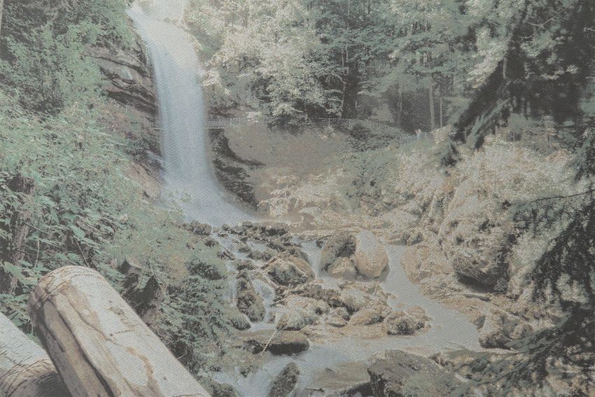
1:2      •   Cucerca, Didyk, Seidel, Babaei

primary colors are then used to mark simple motives and logos.                          This spans a range of laser-marked metals’ behaviors, from elec-
This brute-force color gamut exploration scales poorly with the laser                   tromechanical [Lawrence et al. 2013] to corrosion resistance prop-
marking high-dimensional design space, resulting in neglecting                          erties [ŁeRcka et al. 2016]. More related to our work is a class of
some design parameters.                                                                 studies focused on the effect of various process parameters on the
   The goal of this work is to equip color laser marking with the                       marked colors [Laakso et al. 2009]. Most of these works [Adams et al.
same level of versatility found in color printers. Assuming a black-                    2014; Antończak et al. 2013, 2014] rely on sampling and marking
box model of the difficult device characterization, we design a                         the process parameter space uniformly. As laser marking is time
measurement-based, data-driven performance space exploration.                           and material consuming, these methods cannot cope with the di-
We explore different performance criteria including the color gamut                     mensions of the design space and end up ignoring a large portion
and marking resolution by consecutive marking and measuring. For                        of process parameters. Moreover, we are unaware of any work on
this, we uncover the process’s Pareto front by formulating a multi-                     exploring the marking resolution, separate or jointly by color, a
objective optimization problem and solving it using an evolutionary                     critical performance criterion for high-quality image marking.
algorithm augmented by a Monte-Carlo approach. The optimiza-                               It is worth noting that some empirical color discovery methods
tion explores the hidden corners of our 7 dimensional design space                      [Veiko et al. 2016] try to find different laser parameters that lead
in search of useful parameters that lead to a dense set of diverse,                     to the same color. But that color needs to be known beforehand.
high-resolution colors. We also go far beyond the state of the art                      Moreover, these methods are restricted to interference-based colors
color image marking by introducing a complete color management                          within a limited range of laser energy and a limited number of pa-
workflow that takes an input image and laser-marks the closest                          rameters. This work introduces the first systematic color discovery
approximation on metal surfaces. Our proposed color reproduction                        algorithm for laser marking systems.
workflow adopts the principles of halftone-based color printing. It
extracts a number of primary colors (akin to printer’s inks) from
                                                                                           Performance Space Exploration. In computer graphics, formulating
the explored gamut and reproduces input colors by juxtaposing
                                                                                        design problems based on multi-objective optimization and solving
the extracted primaries next to each other in a controlled manner.
                                                                                        them by computing the Pareto front is known. Notable examples
Our fabricated color images enjoy high resolution, introduce no
                                                                                        are simplifying procedural shaders [Sitthi-Amorn et al. 2011] or
significant artifact, and demonstrate accurate color reproduction.
                                                                                        minimizing power consumption in real-time rendering [Wang et al.
The main contributions of this paper are:
                                                                                        2016] . In computational fabrication, exploring the performance
        • A discovery algorithm that automatically finds the desired                    space (or simply the gamut) of a process has attracted recent at-
          design parameters of a black-box fabrication system.                          tention. With the advent of 3D additive technologies, these efforts
        • The first color-image reproduction workflow for laser mark-                   are mainly focused on exploring the mechanical properties of 3D
          ing on metals.                                                                printed microstructures. As an example, Schumacher et al. [2015]
                                                                                        precompute microstructures’ performance space defined by mechan-
2       BACKGROUND AND RELATED WORK                                                     ical metamaterial families in order to accelerate their heterogeneous
   Color Laser Marking. The coloration of different substrates using                    topology optimization. They first populate the performance space
laser irradiation is an active field of research with a long history                    by perturbing the initial designs (in the design space) and then fill
[Birnbaum 1965]. There are many color formation mechanisms em-                          the unpopulated regions of the performance space through either
ploying different laser sources and different materials; see [Liu et al.                interpolation or inverse optimization. For a similar purpose, Zhu
2019] for a recent review. Surface oxidation is one of these mecha-                     et al. [2017] combine a discrete, random perturbation of designs
nisms where the heat (generated by a laser) facilitates the reaction                    near the gamut boundaries with a continuous optimization that
of materials with oxygen1 . Oxidation-induced colors are believed to                    further expands the gamut by refining existing designs.
stem from multi-layer, heterogeneous mixture of structural colors                          In a more general-purpose method, Schulz et al. [2018] further
(based on thin-film interference) [Del Pino et al. 2004] on one hand,                   emphasize the importance of exploring the performance gamut’s
and the traditional pigment-based color of oxides [Langlade et al.                      hypersurface (or Pareto front) instead of its hypervolume. A Pareto
1998] on the other hand. Despite a handful of initial efforts [Veiko                    front captures a set of solutions in the performance space that are
et al. 2013], predicting the structure and composition of oxide layers                  compromising different, potentially conflicting objectives.
is extremely difficult due to the complex thermodynamics of the                            Although these methods serve as important sources of inspira-
laser marking process [Nánai et al. 1997]. Even with known mate-                        tion, we cannot rely on any of them as they depend on closed-form,
rial composition, predicting the surface color requires a challenging                   smooth characterization functions that connect the design and per-
light-matter interaction model most likely based on an electromag-                      formance spaces. For example, the method of Schulz et al. [2018]
netic simulation [Auzinger et al. 2018]. Based on these observations,                   requires a smooth (twice differentiable) forward characterization
we adopt a black-box model of the process ruling out a physics-based                    of the process and works only with continuous design parameters.
prediction of the laser-induced composition of oxides.                                  Here, similar to Schulz et al. [2018], we cast our performance space
   For some popular metals, such as stainless steel and titanium,                       exploration problem as a multi-objective optimization. But our solu-
oxidation-based color laser marking has been extensively studied.                       tion relies on online marking, measuring of design-space parameters
                                                                                        and navigating it using a modified evolutionary algorithm [Deb et al.
1 The                                                                                   2002].
        same phenomenon turns motorcycles’ exhaust pipes colorful.

ACM Transactions on Graphics, Vol. 39, No. 4, Article 1. Publication date: July 2020.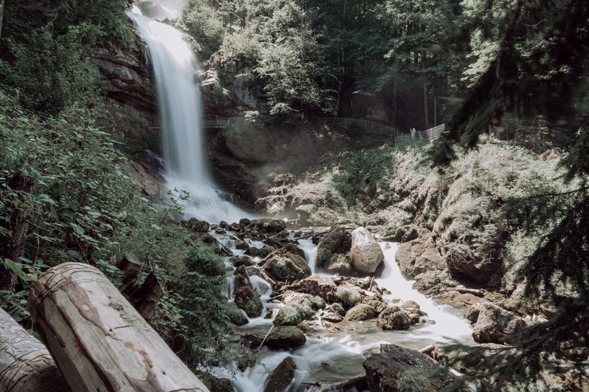
Computational Image Marking on Metals via Laser Induced Heating                         •   1:3

         90                                    90
                                                                                      is shown in Figure 2 where color coordinates of marked patches
         60                                    60                                     may change abruptly in response to marking parameters. It is con-
                                                                                      trasted with the smooth response of a typical printer to its control
CIELAB

         30                                    30
                                                                                      parameters.
          0                                     0
                                                                                          In this section, we propose a non-exhaustive performance space
         -30                                   -30                                    exploration of the laser marking system. Qualitatively speaking, our
               0           0.5           1       100             500            900   performance criteria favors diverse, saturated and high-resolution
                   Cyan area coverage                    Frequency (kHz)              colors: the fundamental requirements for color images. Quantifying
         90                                    90                                     these objectives in Section 3.1, our main insight for solving this
         60                                    60
                                                                                      problem is to cast it as a multi-objective optimization (Section 3.2).
                                                                                      Unlike a typical optimization, multi-objective optimization problems
CIELAB

         30                                    30
                                                                                      are evaluated based on multiple criteria. Very often, these criteria
          0                                      0                                    are in conflict. In our case, for example, some marked colors may
         -30                                   -30
                                                                                      be saturated but leave thick traces and lower the resolution. Hence,
                                                                                      instead of a single optimal solution, there exists a set of optimal
           10        500         1000   1500     20       40           60       80
                                                               Power (%)
                                                                                      solutions, known as Pareto optimal solutions or Pareto set. The pro-
                      Speed (mm/s)
                                                                                      jected Pareto set into the performance space is called Pareto front.
Fig. 2. The color response of our laser vs. that of a a typical printer (top left).   A member of the Pareto front is not dominated by any other point
CIE L*, a* and b* values are plotted in red, green and blue respectively. The         in the performance space in all criteria. In other words, it is more
laser-marked colors (on stainless steel AISI 304) are repeated three times.           performant than all other points in at least one criterion.
Their average (solid lines) and standard deviation (shaded region) are shown.             Our goal is to uncover a dense set of Pareto-optimal solutions to
Notice the non-smooth behavior of the laser-marked colors.                            the color laser marking problem with the above objectives. To this
                                                                                      end, we adopt a multi-objective evolutionary algorithm, a successful
                                                                                      tool for finding Pareto optimal solutions [Fonseca et al. 1993]. The
   Custom Color Reproduction. Our work is closely related to color                    algorithm, called non-dominated sorting genetic algorithm (NSGA-
printing as our final objective is to reproduce color images through                  II) [Deb et al. 2002] is well suited to our model-free characterization
laser marking. Color reproduction, to the best of our knowledge,                      function, with both discrete and continuous parameters. At the
is absent in the laser marking literature. The closest practice is to                 heart of this method, is a sorting algorithm based on the members’
mark simple logos and motives without systematic reproduction in                      presence in multi-level Pareto fronts. As we show, the NSGA-II
mind. Our goal is to start from a source image (e.g., sRGB) and mark                  non-dominated sorting is insufficient for our specific problem due
its most accurate approximation on metals using a custom color                        to our hue diversity objective. Thus, we resort to a Monte-Carlo
reproduction workflow. While the traditional color reproduction                       approach on top of the non-dominated sorting and introduce a new
workflow is well validated for printing inks on paper, it falls short                 sorting method based on front frequencies. We call this algorithm
when dealing with unconventional circumstances, such as non-                          Monte-Carlo, multi-objective, genetic algorithm or MCMOGA for
standard inks [Hersch et al. 2007] or substrates [Pjanic and Hersch                   short.
2013]. In such circumstances, custom color reproduction pipelines
are required [Stollnitz et al. 1998]. We find these custom workflows                  3.1    Color Laser Marking Performance Criteria
to fit well to the problem at hand. In particular, as we will show
                                                                                      As we plan to adopt halftoning for color reproduction (Section 4.2),
in Section 4, the juxtaposed halftone color reproduction workflow
                                                                                      we need a set of primary colors that cover both achromatic and
can be adapted to our color reproduction setup. This workflow is
                                                                                      chromatic axes. In a divide and conquer strategy, we separate the
designed to print with opaque inks and includes juxtaposed halftone
                                                                                      chromatic and achromatic (black and white) explorations, starting
synthesis [Babaei and Hersch 2012], color prediction [Babaei and
                                                                                      here with explaining the former. High chromatic performance re-
Hersch 2016a] and color separation [Babaei and Hersch 2016b].
                                                                                      quires saturated colors corresponding to larger radii in the CIECH
                                                                                      color space shown in Figure 4 [Schanda 2007]. Furthermore, it re-
3          GAMUT EXPLORATION
                                                                                      quires colors that span a range of different hues. Such colors mixed
Device characterization is the prerequisite for any color reproduc-                   with black and white (through halftoning) generate a highly popu-
tion system including laser marking. In the absence of an analytical                  lated color gamut that can be utilized for color image marking.
function that maps laser marking parameters to marked colors, we                         The goal of our multi-objective optimization is to, eventually,
must rely on data-driven methods. In a first attempt, one can sample                  maximize the following criteria:
the design space, mark and measure the sampled design points, and
                                                                                         (1) Chromaticity, as marked colors with large chroma produce
construct a look-up table. This exhaustive strategy is subject to the
                                                                                             more saturated color images.
curse of dimensionality given the relatively large number (7) of
parameters involved in color laser marking. The fact that function
                                                                                                                             p
                                                                                                            fC (a ∗ , b ∗ ) = a ∗2 + b ∗2          (1)
evaluations require actual marking and measuring further slows
down the process. Additionally, the non-smooth color response to                              where a ∗ and b ∗ are the color coordinates of the CIELAB
laser parameters renders interpolation schemes ineffective. This                              color space [Wyszecki and Stiles 1982].

                                                                                       ACM Transactions on Graphics, Vol. 39, No. 4, Article 1. Publication date: July 2020.
1:4 • Cucerca, Didyk, Seidel, Babaei
ons
u t
s
ing
am
e
lati
r
asu
r
to g
opu
ffsp
me
ep
te o
Add
nd
bin
S
era
MO
rk a
⑤
Com
Pi Gen Qi Qi Ri Ri
MC
DS PS
Ma
③
②
①
④
hal er
P i +1
⑥ Fitt
f
GA Pi U Q i
DS PS DS DS PS DS PS DS PS
DS PS
Fig. 3. One iteration of MCMOGA. ○ 1 The algorithm takes the starting population at iteration i (Pi ) and uses the genetic algorithm to generate an offspring
generation Qi . ○
2 Marking and measuring the design space (DS) yields the corresponding points in the performance space (PS). Pi and Qi are combined into
Ri ○3 and sorted using the proposed MCMOS algorithm ○. 4 Ri is added to the gamut ○ 5 and its fitter half Pi+1 is passed as the starting generation to the next
iteration ○.
6
(2) Hue spread (f HS ) ensures the presence of high-chromaticity GA and used to create the next generation. Given the difficulty of
colors at all hue angles. assigning a single fitness value to multi-criterion objectives, the non-
(3) Resolution; since we use a line-based halftoning, this criterion dominated sorting algorithm [Deb et al. 2002] sorts the members of
is evaluated by measuring the thickness of a line marked by a population according to their presence in multi-level Pareto fronts
a set of given laser parameters. (Appendix B). It starts with finding the first non-dominated front,
1 i.e., all solutions in a population that belong to the Pareto front.
f R (t) = (2) This is done by comparing each solutions’ performance objective
t
where t is the line thickness. by objective to every other solution in the population. If a solution
(4) Performance space diversity (PSD); it is measured for each is more performant than all other solutions in at least one criterion,
point in the CIECH space as the reciprocal of the distance to it is labeled as a first-front solution. The second non-dominated
its closest two neighbors. front is computed by temporarily discarding the first front and re-
peating the above procedure. This procedure is continued until all
1 members of the population are labeled with their respective fronts.
f PSD (p, P) =
argmini, j ∥p − Pi ∥ 2 + ∥p − P j ∥ 2 (3) This results in a number of disjoint subsets making up the whole
i , j, 0 ≤ i, j < |P | population, each with its front label. Note that, in the spirit of the
Pareto concept, members inside the same front are not sorted.
where p is the point to be scored and P its respective popula-
This type of sorting is not sufficient when considering the hue
tion in CIECH space.
spread objective. This criterion helps the color gamut grow in all
(5) Design space diversity (f DSD ); it is measured as the perfor-
angular directions in a balanced manner. Without the hue spread
mance space diversity except in the design space.
criterion, the algorithm may explore some specific hue angles more
Criteria (1) to (4) are measured in the performance space while than others resulting in a non-uniform growth of the chromaticity
criterion (5) is measured in the design space. Criteria (1) to (3) are the gamut. For achieving a gamut with balanced hue spread we cannot
qualities we are directly seeking for laser marked images. Criterion evaluate a single solution but rather in combination with other
(4) improves the convergence rate and criterion (5) helps avoiding solutions. This can quickly lead to nontrivial computation: for 10
local extrema by promoting solo points in the performance space. angular samples in a population of 200, we must perform 200 10
≃
3.2 Monte-Carlo Multi-objective Genetic Algorithm 1016 evaluations.
We avoid this combinatorial explosion by resorting to a Monte-
Our algorithm, navigates the laser’s design space in directions that Carlo method. A hue wheel splits the CIECH space into a random
lead to a dense Pareto set, i.e., the set of designs (laser parame- number of circular sectors (Figure 4). Within each sector, we sort
ters) that improves the above performance criteria. We start with the solutions using the described non-dominated sorting algorithm
a random population in the design space, mark it and measure its based on all criteria except the hue spread. We repeat this procedure
performance, then iteratively evolve it into a larger population with each time with a randomly chosen number of sectors, and with
as many Pareto optimal solutions as possible. At each iteration, a random angular offset. After each turn of the hue wheel, every
represented schematically in Figure 3, we promote the Pareto set individual solution is assigned to a potentially different front. At the
of its population to be passed along to the next iterations using end of this loop, every single solution is characterized by its front
the genetic algorithm. We stop iterating when we do not observe a frequency vector that represents the frequency of its presence in
significant improvement in the Pareto front. the first front, second front and so on. We stop "turning" the Monte-
3.2.1 Monte-Carlo Multi-objective Sorting. As in almost any ge- Carlo hue wheel when the change in front frequencies is below a
netic algorithm (GA) method, a fitness measure should be assigned certain threshold. The population is sorted based on the frequency
to each member of the population. Fitter solutions are selected by of their "top" fronts where a single first front is worth more than any
ACM Transactions on Graphics, Vol. 39, No. 4, Article 1. Publication date: July 2020.
Computational Image Marking on Metals via Laser Induced Heating                         •   1:5

      Hue wheel 1            Hue wheel 2
                                                                                           Algorithm 1: Monte-Carlo multi-objective sorting (MCMOS)
              ② ①                  ②
                                                                                               Input
                             ①
                                                                                          1
      ①                                    ①                                              2        P : Population
          ②                 ②                          Front frequencies
                      *③                   *③                                             3        ≺ : Partial order on P
      ①                                                                                            t : Stopping threshold
                             ③
                                                                                          4
                  ②                        ②
          ① ②                 ① ②
                      ①                                          (2|2|0)
                                                                                          5        α lim : Offset limits for hue wheel
                                                       (4|0|0)
                                       ①                                   (3|1|0)        6        C #lim : Limits for number of circular sections
                                                    (1|3|0)                               7    Output
                                                                                (2|0|2)
      Hue wheel 3            Hue wheel 4
                                                   (3|0|1)
                                                                            *             8        P s : Sorted population P
                                                                           (0|4|0)        9    Procedure
                                                    (4|0|0)      (0|3|1)
       ①      ①                   ①                                                            begin
                            ①
                                                                                          10
                    ①                      ②                          (4|0|0)                      // Initialize front frequencies with 0
                            ②
                                                                                          11
      ①                                     ①
                    *①                     *                                              12       Θ ← 0;
      ①                     ①                                                             13       // Initialize frequencies difference
              ③②                           ②
          ①                     ① ②                                                       14       ∆Θ ← ∞;
                ①                      ①                                                  15       // Initialize prior front frequencies
                                                                                          16       Θpr ← Θ;
                                                                                          17       while (∆Θ > t ) do
Fig. 4. Examples of different hue-wheel configurations (left) used in MC-                 18              // Draw hue wheel parameters
MOS. First, the points within each circular sector of each hue wheel are                  19              α ← random(α lim );
assigned to front labels (encircled numbers next to each point) using the                 20             C # ← random(C #lim );
conventional NDS algorithm. Next, all front labels for each point are counted             21              // Split population into circular sections
to form the front frequencies (right). As an example, the point shown with                22             C ← HueWheel(P , α , C # );
a star has been assigned two times to the first front and two times to the                23              // Iterate over circular sections
third front. Notice that, for the same point, only the first two hue-wheels               24              for c ∈ C do
                                                                                          25                   // Compute front indices
would not suffice as it would have been assigned only to the third front                  26                   δ ← NDS(c , ≺);
despite high potential for improving the gamut.                                           27                   // Update front frequencies
                                                                                          28                   Θc, δ ++;
                                                                                          29              end
number of second fronts. This procedure is schematically shown in                         30              // Compute change in front frequencies
Figure 4. Note that multiple turns of the hue wheel, with different                       31              ∆Θ ← ∥Θ − Θpr ∥F ;
                                                                                          32              // Cache front frequencies state
number of sectors and angular offsets, ensure all points are sorted in                    33              Θpr ← Θ;
different configurations and are ranked in a proper way. In Figure 4,                     34       end
for example, it is easy to see that some points may not be sorted                         35       // Sort points according to front frequencies
properly using a single hue-wheel configuration. The pseudo-code                          36       P s ← Sort(P , Θ);
                                                                                               end
for the sorting algorithm, called Monte-Carlo multi-objective sorting                     37

(MCMOS), is shown in Algorithm 1.
   3.2.2 Achromatic Exploration. In our chromatic exploration, the                        smaller number of primaries lead to improved marking time as they
lightness values (CIE L∗ ) are discarded. We perform two separate                         cause fewer switching delays (Section 5.1.1). Not all colors in the
explorations for black and white colors on the lightness axis. For                        explored gamut can be considered for primary extraction. Thus,
the black colors, we minimize the criteria (1), thereby encouraging                       before primary extraction, we prune the gamut by excluding colors
low chromaticity colors, and replace criterion (2) with lightness                         that: 1) don’t satisfy our specified resolution requirement, 2) reveal
minimization. Exploring white colors is the same as the black colors                      low repeatability, and 3) exhibit non-uniformity.
except in (2) we maximize the lightness.                                                     Similar to the gamut exploration, we extract the achromatic and
                                                                                          chromatic primaries separately. We start with the explored chro-
4     IMAGE REPRODUCTION                                                                  maticity gamut of the laser marking system composed of a discrete
Once the performance space of our laser marking system is explored,                       set of colors. We find the convex hull of this set in the CIExy chro-
it can be exploited for color image reproduction. We propose to                           maticity space where x = X /(X + Y + Z ), y = Y /(X + Y + Z )
adopt the principles of halftone-based color printing for color laser                     [Wyszecki and Stiles 1982]. The reason for applying the convex
marking. For this, we find a number of primary colors (equivalent                         hull in the CIExy is that, unlike CIEa*b* or CIECH, it is a linear
to printer’s inks) that meet our resolution requirement and produce                       space under halftoning. We experimentally confirm this linearity in
the largest color gamut (Section 4.1). We then build a color manage-                      Section 5.3, where we show that colors inside the convex hull can be
ment workflow that takes input color images and marks the closest                         reproduced through halftoning with high accuracy. The colors in the
approximation using the selected color primaries (Section 4.2).                           convex set give the largest area and therefore the largest chromatic
                                                                                          gamut. In order to reduce the number of primaries, we can further
4.1    Primary Extraction                                                                 exclude those members of the convex set that don’t contribute to the
The primary extraction is concerned with selecting a set of colors                        gamut area significantly. The achromatic primary extraction selects
that generates the maximum color gamut through halftoning. While,                         the darkest and the brightest colors with negligible chromaticity
unlike printers, the number of primaries is not strictly limited, a                       from within the black and white explored gamuts, respectively.

                                                                                           ACM Transactions on Graphics, Vol. 39, No. 4, Article 1. Publication date: July 2020.
1:6   •    Cucerca, Didyk, Seidel, Babaei

                                                                                        raster devices, we need to transform the resulting raster images into
                                                                                        vector representation suitable for our laser device. For this purpose,
                                                                                        we use a naive line (a discrete line with unit thickness) as a mask
                                                                                        and slide it on each halftone layer corresponding to each laser pri-
                                                                                        mary (Figure 5). This produces a list of vectors of different primaries
                                                                                        which span the image plane and are sent to the laser device for
                                                                                        marking.
                                                                                            4.2.2 Forward Color Prediction. The color prediction model has
Fig. 5. Laser marking’s color reproduction workflow. ○ 1 An input image is              two roles in our proposed color management workflow. First, it
mapped to the gamut of the laser marking system. ○ 2 In the color separation            constructs the color gamut generated by halftoning a set of primaries.
step, for each mapped color, the corresponding area coverages of each                   It predicts the color of several thousands of halftones spanning the
primary is computed (creating the gamut and color separation are built upon             space of the relative area of primaries in each halftone, known as
a color prediction model). ○
                           3 The continuous area-coverages are binarized                area coverages. The gamut surface is then fitted to this volumetric
and placed next to each other using a juxtaposed halftoning method. ○ 4 The             point cloud and is later used for gamut mapping. Second, the forward
raster halftone images are converted into vectors.                                      model is used in the color separation step that computes the area
                                                                                        coverages of the primaries for any input colors to be reproduced.
                                                                                           We use the Yule-Nielsen (YN) prediction model to predict the
4.2    Color Management Workflow                                                        multi-color, juxtaposed halftones of laser primaries. The Yule-Nielsen
A color management workflow ensures color reproducibility across                        equation [Yule and Nielsen 1951] predicts the CIEX color coordinate
different imaging devices. The classic example is printing where the                    (X t ) of a juxtaposed halftone as
input images, from a camera for example, are printed as accurately
                                                                                                                       q
as possible. Figure 5 sketches our proposed color reproduction work-                                                                        n
                                                                                                                             ai (X i )1/n
                                                                                                                      Õ
flow for color laser marking. Given an input color in a given color                                            Xt =                                         (4)
                                                                                                                       i=1
space, e.g., sRGB, we first ensure its reproducibility by mapping it
                                                                                        where X i is the CIEX value of the i-th primary, and ai is its area
into the color gamut of laser marking. The color separation com-
                                                                                        coverage. The same equation applies for predicting CIEX and CIEY
putes the coverage of different laser primary colors which, when
                                                                                        color coordinates. The exponent n, called the Yule-Nielsen n-value
placed next to each other through halftoning, reproduce the input
                                                                                        is a tuning parameter which we further discuss in Section 5.3.
color.
   A typical printer’s color reproduction workflow generates differ-                       4.2.3 Color Separation. Color separation builds on the forward
ent colors by spatial blending and superposition of multiple inks.                      prediction model to compute the particular primaries and their area
Should we imitate such a workflow for the laser marking process,                        coverages that reproduce a given color (inside the color gamut).
we would need to ensure both laser primaries and their superposi-                       As the YN model is not analytically invertible, color separation is
tions are optimal. Exploring the design space for such an unlikely                      carried out by optimization:
combination is significantly more difficult. Instead, we propose to                                        argmin ∆E 00 Lab(YN(a)), c

place different primaries strictly next to each other resulting in a                                          a                                          (5)
considerably simpler exploration where we search only for a set of                                               ∥a∥ 1 = 1, a ∈ [0, 1]q
suitable primaries (and not their superpositions). We build on an
                                                                                        where c is the target color in the CIELAB color space and a is the
existing juxtaposed halftoning reproduction workflow [Babaei and
                                                                                        optimization variable, i.e. the vector of area coverages of q primaries.
Hersch 2012] developed for the color reproduction of opaque inks.
                                                                                        As the CIEDE2000 color-difference formula [Sharma et al. 2005] is
In order to establish such a workflow, we synthesize juxtaposed
                                                                                        used for the distance metric, the modeled color using the YN model
halftones of extracted primaries (Section 4.2.1), predict the integral
                                                                                        (YN(a)) should be converted to CIELAB from CIEXYZ (denoted by
color of multi-primary halftones (Section 4.2.2), and numerically in-
                                                                                        function Lab in Equation 5). Equation 5 searches for an area coverage
vert this prediction model in order to map input colors into primary
                                                                                        vector that, after being marked, results in the minimum distance to
halftones (Section 4.2.3).
                                                                                        the target color. As we juxtapose different primaries, their relative
   4.2.1 Juxtaposed Halftoning. Color halftoning converts a con-                        area coverages should sum up to 1 and be non-negative.
tinuous tone color image into a set of binary images each corre-
sponding to one of the printer’s inks. The discrete-line juxtaposed                     5     RESULTS AND ANALYSIS
halftoning [Babaei and Hersch 2012] synthesizes these binary im-                        In this section, we present different analyses and evaluations of both
ages in the form of lines and places them next to each other without                    gamut exploration and image reproduction.
overlapping. In the original algorithm designed for bitmap printers,
using digital lines [Reveilles 1995] allows for subpixel thickness,                     5.1    Experimental Setup
low computational complexity, and, importantly to us, continuity. A                        5.1.1 Laser Marking Hardware and Parameters. We assemble a
continuous laser path ensures less switching delays, and therefore,                     laser marking device (Figure 6) whose main components are a ytter-
faster marking with lower graininess caused by the two ends of each                     bium fiber laser system (IPG Photonics YLPM-1-4x200-20-20) and a
marked vector. As the original juxtaposed halftoning is designed for                    galvanometric scanner (Scanlab IntelliScan III 10). The laser system

ACM Transactions on Graphics, Vol. 39, No. 4, Article 1. Publication date: July 2020.
Computational Image Marking on Metals via Laser Induced Heating • 1:7
Speed
y
nc
eq 1
th
ue
Hatching
id
w
Pulse energy
Fr
lse
Line count
Pu
t
un
co
Time
ss
er
Pa
Las er
a nn
Sc Fig. 7. Visualization of laser (left) and scanner (right) parameters. The multi-
n
tio
tila pass line cluster in the diagram on right forms the final color.
Ven e
t
stra
Sub
e
tag
Z-S
delays after changing these parameters ensuring the laser source
can properly adapt to the new parameters.
5.1.2 Performance Space Measurement. For each point in the
design space, we need to measure its performance in order to decide
Fig. 6. Our assembled laser marking device with annotated modules.
how to use that point in our exploration framework. All performance
criteria, apart from the design space diversity, can be evaluated by
measuring the thickness of a marked line cluster and the color of
(20 W, 1064 nm) generates a laser beam which is redirected by the a marked patch. This is performed in two stages. First, for measur-
scanner’s Galvo Mirror system to any desired spot on the substrate. ing the cluster’s thickness, we use a hand-held digital microscope
Equipped with an infrared F-Theta lens (f=163 mm), the scanner (Reflecta DigiMicroscope USB 200). In a second step, we use the
is capable of imaging a planar field of 116 × 116 mm. For safety thickness of a given cluster to mark its corresponding patch by
reasons, the whole laser marking system is covered in an enclosure juxtaposing multiple clusters within the desired area.
within which the laser source is separated by aluminum plates. An Both hue and chromaticity, the pillars of our performance space
air filtering system blocks small particles from spreading in the exploration, are computed from CIELAB, a perceptual color space.
room. In most of our experiments we use 1 mm thick stainless steel We therefore perform a colorimetric calibration [Hong et al. 2001] for
type 1.4301 V2A (AISI 304) as a substrate. We use thicker substrates measuring the color of marked patches. The colorimetric calibration
and another stainless steel alloy (AISI 430) in some experiments connects camera RGB signals to CIEXYZ coordinates through a
in Section 5.4. Note that color laser marking is also possible on form of regression. The CIEXYZ values then can be converted to
titanium. the CIELAB coordinates using a set of well-known, analytical trans-
In this work, we study 7 marking parameters (Figure 7), including formations [Wyszecki and Stiles 1982]. For training the regression,
laser parameters: we use 121 printed color patches, with known spectra measured
(1) Frequency: Defines the number of laser shots per second (1.6- with an X-Rite i7 spectrophotometer, and obtain the ground-truth
1000 kHz, 100 Hz steps), CIEXYZ values assuming D65 illumination.
(2) Power: Adjusts the output power per shot (0-100%, 256 steps), We capture the same printed patches with a Nikon D750 DSLR
(3) Pulse width: Defines the duration of a single shot (4, 8, 14, 20, camera (with macro lens Tamron SP 90mm F/2.8 Di) obtaining raw
30, 50, 100, 200 ns), RGB signals that have been corrected for spatial and temporal light
fluctuations. Our colorimetric calibration shows high accuracy on
and scanning parameters that forms a line cluster with properties: a test set of 16 printed patches with an average ∆E 00 = 2.26 and
(4) Speed: Defines the travel speed along a vector while marking maximum 5.00. This calibration is therefore used to estimate the
(0-2000 mm/s, 1 mm/s steps), CIELAB color of marked patches.
(5) Line count: Defines the number of lines in a cluster (1-20 lines, The structural nature of oxide colors causes a significant change
1 line steps), in their appearance depending on the viewing and illumination
(6) Hatching: Defines the distance between lines within a cluster geometry. We observe that laser-marked colors appear most satu-
(1-15 µm, 1 µm steps), rated at specular and near-specular geometries. Therefore, inspired
(7) Pass count: Indicates the number of times a vector is marked by previous work on metallic prints [Pjanic and Hersch 2013], we
(1-10 passes, 1 pass steps). confine our color reproduction to non-diffuse geometries. To this
It is worth noting that, due to technical limitations of the laser end, the stainless steel substrate is illuminated with a large, diffuse
source, laser parameters cannot be used at arbitrary combinations. area-light tilted approximately 45◦ from the substrate’s normal and
Furthermore, it is not possible to vary laser parameters on the fly. captured with the camera with a similar angle.
For example, switching frequency and power takes 0.6 ms and 3 ms
respectively; changing the pulse width takes about 2 seconds as it 5.2 Gamut Exploration Evaluation
requires reestablishing the connection between the controller board For evaluating the proposed gamut exploration algorithm, we per-
and the laser. In our path planning, we therefore allow switching form multiple runs while discarding different objectives during
ACM Transactions on Graphics, Vol. 39, No. 4, Article 1. Publication date: July 2020.
1:8   •    Cucerca, Didyk, Seidel, Babaei

                                                                                        Average t (in μm)
                                                                                                            55                                        12                              0.4

                                                                                                                                            E 00
                                                                                                                                                      9

                                                                                                                                                                              CIE y
                                                                                                            45                                                                        0.35

                                                                                                                                            Average
                                                                                                                                                      6
                                                                                                            35                                        3                               0.3

                                                                                                                 0     5      10 15    20                  -2 -1 0 1      2             0.25   0.3        0.35   0.4
                                                                                                                           Iteration                           n -value                              CIE x

       (a) I=0              (b) I=10             (c) I=30             (d) I=50                                             (a)                               (b)                               (c)

Fig. 8. Color gamut evolution of a full exploration (with fC , f HS , f R , f PSD ,     Fig. 11. (a) Average thicknesses over iterations with (continuous line) and
f DSD ) on AISI 304 stainless steel.                                                    without (dashed line) f R (only t < 80 µm were considered). (b) Average
                                                                                        reproduction error of the Yule-Nielsen model for different n-values. (c)
                                                                                        Extraction of chromatic primaries.

                                                                                           Comparison with Random Marking. We compare the gamut of a
                                                                                        set of randomly marked patches (Figure 9) with the results of our
                                                                                        exploration. Compared to our full exploration (Figure 8), random
       (a) I=0              (b) I=5              (c) I=10             (d) I=20          marking does not lead to adequate gamut growth. As the random
                                                                                        exploration does not include the resolution objective, it is more
Fig. 9. Color gamut evolution of a random exploration on AISI 304 stainless             illustrative to compare Figure 9d to Figure 10e as they both feature
steel.                                                                                  the same number of samples and none of them includes the resolu-
                                                                                        tion objective. The stagnant behavior of random marking over time
                                                                                        (Figure 9) and a lack of systematic resolution enhancement suggest
                                                                                        that a very large number of samples is required to match the full
                                                                                        gamut generated by our algorithm.
                                                                                           Effect of Monte-Carlo Hue Wheel. In order to evaluate the effective-
                                                                                        ness of our Monte-Carlo hue wheel algorithm, we run two similar
                                                                                        explorations where the only difference is that the hue-spread objec-
              (a) With f HS           (b) With f R       (c) With f R
                                                                                        tive f HS is enabled in one (Figure 10a) and disabled in the second
           (without f R ) (I=10)         (I=20)        (I=20, t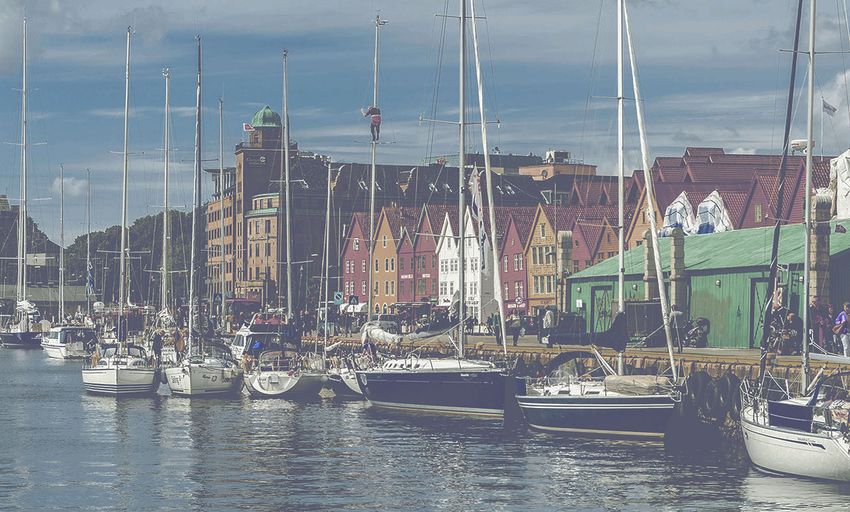
Computational Image Marking on Metals via Laser Induced Heating                            •   1:9

Fig. 12. Multiple examples of original (left), gamut mapped (center) and marked images (right). The marked images, on AISI 304 stainless steel, are photographed
in the non-diffuse mode. Images © Sebastian Cucerca, Steve Johnson, Albrecht Dürer, Vahid Babaei.

   Primary Extraction. After the pruning step discussed in Section 4.1,            showed that this parameter is responsible for shadowing and mask-
we obtain a total of 6 primaries including a black and white primary               ing in metallic-ink halftones. From the optimal n-value for our setup
and 4 chromatic primaries shown in Figure 11c. Their parameters                    we can infer that, as expected, the subsurface scattering in metal is
are reported in Appendix A. In the pruning stage, we check the spa-                very negligible. Furthermore, the marked primaries are very well
tial and temporal repeatability by marking the candidate primaries                 leveled on the surface and cause no shadowing or masking.
at four different locations of the substrate and compare their colors
pairwise. Primaries having an average ∆E 00 higher than 4 among                       Marking Color Images. Figure 12 presents different results gener-
all comparisons are discarded. Also for the progressive primary                    ated by the proposed image reproduction pipeline with the chosen
discarding, we reduce the number of primaries until the gamut area                 primaries. Comparing the marked images with their gamut-mapped
drops by more than 10%. For resolution pruning, in this work, we                   counterparts, we can observe that the colors are reproduced faith-
keep colors with thickness 40 ± 5 µm. Additionally, we consider                    fully. Furthermore, no significant artifacts are introduced in the
colors with thickness around 20 µm as juxtaposing two of them                      laser-marked images. The gamut of the primary set allows marking
results in the target resolution.                                                  diverse, vivid and relatively saturated colors as pointed by the image
                                                                                   in the second row of Figure 12. Thanks to the high-resolution pri-
                                                                                   maries, high spatial frequencies are preserved. This allows marking
   Prediction Model Accuracy. For testing the accuracy of the Yule-                images with a vast level of details as shown in the bottom-right row
Nielsen model, we mark the primaries and also 92 test patches with                 of Figure 12.
diverse area coverages of primaries. The resulting average ∆E00
error is 2.25 (Std=0.96, Min=0.50, Max=4.26) that demonstrates the                 5.4    Repeatability and Generalizability
high accuracy of our forward model. As we show in Figure 11b, the
                                                                                   In this section, we study the question of whether the marking pa-
n-value equal to 1 works very well for our configuration, reduc-
                                                                                   rameters are transferable when using different marking settings
ing our model to the widely known Neugebauer model [Rolleston
                                                                                   or substrates. We start by marking a set of parameters reported in
and Balasubramanian 1993]. There are a handful of physical and
                                                                                   literature [Antończak et al. 2013] and show the results in Figure 13.
empirical interpretations of the Yule-Nielsen n-value in literature
                                                                                   Despite using highly similar hardware and materials, the reported
[Lewandowski et al. 2006]. In the classic ink-on-paper prints, it
                                                                                   colors are not reproducible on our setup. Also, color thicknesses vary
accounts for the optical dot gain due to the lateral propagation of
                                                                                   significantly making them unsuitable for halftoning and therefore
light inside the substrate [Hébert 2014]. Babaei and Hersch [2015]
                                                                                   image marking.

                                                                                    ACM Transactions on Graphics, Vol. 39, No. 4, Article 1. Publication date: July 2020.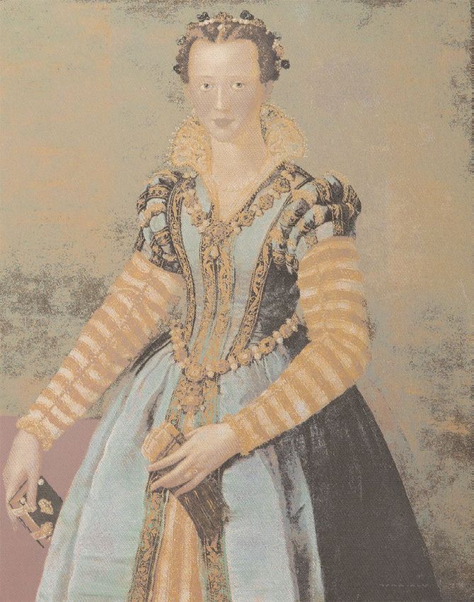
1:10    • Cucerca, Didyk, Seidel, Babaei

            Closest color
            in our gamut

         Antończak et al.

            Marked with
            our hardware
        (thickness in μm) (23)     (217)   (66)    (132)   (70)   (613)     (94)   (252)

Fig. 13. Marking parameters from Antończak et al. [2013], resulting in colors
shown in the middle row (as reported in the original paper). Same parameters
marked on the same material (AISI 304) using our device (bottom) lead to
significant color differences (mean ∆E 00 = 15.3) and a huge thickness
variation. We also show (top) the closest colors in our gamut to the reported
colors in the middle.

   In Table 1, we report color differences when marking on our setup
                                                                                           Fig. 14. Marked images on AISI 304 (top left) and AISI 430 (top right) with
a general set of parameters in different circumstances. The general
                                                                                           the same primaries explored and extracted on AISI 304. A newly explored
set, consisting of 89 design points, is chosen to represent different                      and extracted set of primaries on AISI 430 are used for marking an image:
colors in our explored gamut. We can see a pure repeatability test, on                     gamut-mapped (bottom left) and photograph (bottom right). Image © Piotr
AISI 304 alloy, using the same marking settings leads to acceptable                        Didyk.
but not satisfactory accuracy. When we change the marking settings
by using a thicker substrate (2 mm), and therefore exiting the focal
plane, the repeatability worsens. Finally, using a different alloy of
stainless steel (AISI 430) results in the worst repeatability.
   For comparison, in Table 1, we also show the result of the same
experiments performed using our 6 extracted primaries. We observe
significantly higher accuracy in the pure repeatability experiment as
the primaries have been pruned against this circumstance. Interest-
                                                                                                  (a) I=0             (b) I=10            (c) I=30             (d) I=50
ingly, the primaries show acceptable repeatability when marked out
of focus indicating that the extracted primaries are robust against
                                                                                           Fig. 15. Color gamut evolution of a full exploration (with fC , f HS , f R , f PSD ,
some perturbations. However, the larger deviation when using a new
                                                                                           f DSD ) on AISI 430 stainless steel.
substrate suggests that the primaries cannot be used for marking
images on new substrates accurately.
   In Figure 14, we mark an image on a new substrate (stainless steel                      measuring their thicknesses with a handheld microscope, marking
AISI 430) using primaries explored and extracted on our default                            the corresponding patches with proper distances of clusters, and
substrate (AISI 304). While the image on the new substrate preserves                       finally capturing them with our colorimetric camera. The manual
the spatial details, most colors are significantly paler compared to the                   measurement of cluster thicknesses is the bottleneck as it takes
image marked on the default substrate. Thus, we perform a complete                         approximately 20 minutes. Computing a new generation using the
gamut exploration, primary extraction and color reproduction on                            MCMOGA takes only a few seconds in Matlab.
the new substrate and show the results in Figure 14 (bottom row).                             The marking time of an image is a function of the number of vec-
Note that we cannot expect the same reproduction as on the default                         tors (after halftone vectorization) and the marking speed of different
substrate since the color gamuts on two substrates are different.                          primaries. A larger number of vector causes more switching delays,
The gamut of the new substrate, calculated using a full exploration,                       making the marking time highly dependent on the image content in
is shown in Figure 15 (gamut obtained on the default substrate is                          addition to its size. For example, the two marked images in the top
shown in Figure 8).                                                                        row, and right side of the bottom row of Figure 12, despite a com-
                                                                                           parable image size (7 by 11 cm), required around 18 and 30 million
Table 1. Repeatability errors of color laser marking in form of ∆E 00 mean                 vectors, and roughly 3 and 5.5 hours of marking time, respectively.
(and standard deviation).
                                                                                           6    CONCLUSION
          Substrate A       AISI 304            AISI 304                   AISI 304        We presented a computational framework that enables a novel ap-
          Substrate B       AISI 304       2 mm thick AISI 304             AISI 430
                                                                                           plication of laser marking: color image reproduction. Our method
          General set       5.42 (5.63)           9.30 (6.27)             16.37 (7.50)
           Primaries        1.96 (2.06)           6.46 (4.15)             12.33 (7.25)     first characterizes the device using an evolutionary exploration of
                                                                                           its performance space and then exploits that space for marking
                                                                                           high-resolution, colorful images.
5.5    Performance                                                                            Pitfalls, Limitations and Outlook. Proper imaging was a challeng-
An iteration of the gamut exploration with a population size of 100                        ing part of this research. We started the colorimetric calibration
takes around 30 minutes. This includes marking the single clusters,                        of the camera using the spectra of laser-marked patches (and not

ACM Transactions on Graphics, Vol. 39, No. 4, Article 1. Publication date: July 2020.
Computational Image Marking on Metals via Laser Induced Heating • 1:11
B NON-DOMINATED SORTING ALGORITHM
The non-dominated sorting (NDS), depicted in Algorithm 2, com-
putes the front indices of population members. We refer the reader
to Deb et al. [2002] for further details.
Algorithm 2: Non-dominated Sorting Algorithm
1 Input
2 P : Population
3 ≺ : Partial order on P
4 Output
Fig. 16. Image marked on AISI 304 and captured in non-diffuse (left) and 5 δ : Front indices
diffuse (right) modes. Painting © Alessandro Allori. 6 Procedure
7 begin
printed colors on paper). Although our spectrophotometer can per- 8 for (p ∈ P ) do
S p ← ∅;
form measurements that include the specular component, the mea- 9
10 np ← 0;
sured spectra were inconsistent with reality. Fortunately, switching 11 for (q ∈ P ) do
to the printed colors for calibrating the colorimetric characterization 12 // Check if p dominates q
proved to be robust. Another imaging-related issue was measur- 13 if (p ≺ q ) then
14 // Add q to points dominated by p
ing the thickness of the clusters using a camera. The efforts were 15 Sp ← Sp ∪ {q };
not successful and led to the use of a handheld microscope that 16 else if (q ≺ p ) then
significantly slowed down our exploration. 17 // Increase domination counter of p
A clear limitation of our method is the significant change of ap- 18 np ← np + 1;
19 end
pearance from diffuse to non-diffuse configurations as shown in 20 end
Figure 16. While amusing, producing plausible images in a wider 21 if (np = 0) then
range of viewing/illumination geometries is an important research 22 // p is in front 1
direction and a formidable challenge. In the future, we plan to ana- 23 δ ← 1;
24 F 1 ← F 1 ∪ {p };
lyze the performance of our method in the case the pruning stage 25 end
is integrated into the exploration using new objectives. We inten- 26 end
tionally did not consider the physical phenomena behind the laser 27 // Initialize front counter
marking and stayed with a black-box approach. Yet we believe a 28 i ← 1;
while (F i , ∅) do
combination of both physical and data-driven methods can make 29
30 // Set storing next front’s members
the color image marking task more scalable. 31 Q ← ∅;
32 for (p ∈ F i ) do
A PRIMARY PARAMETERS 33 for (q ∈ Sp ) do
34 nq ← nq − 1;
The design and performance space parameters of the extracted set of 35 if (nq = 0) then
primaries are shown in Table 2. In the project’s website, we also pub- 36 // Add q to next front
lish the intermediate exploration data, i.e., design parameters and 37 δ q ← i + 1;
Q ← Q ∪ {q };
performance measurements for all marked patches at all iterations
38
39 end
of our full exploration. 40 end
41 end
Table 2. Design and performance space parameters of extracted primaries 42 i ← i + 1;
on AISI 304 (top segment) and AISI 430 (bottom segment). 43 Fi ← Q ;
44 end
45 end
Frequency Power Pulse Speed Line Hatching Pass CIELAB t
width count count
kHz % ns mm/s # µm # L*, a*, b* µm
650.7 29.5 20 1897 7 2 6 64.4, -15.9, -0.3 21
887.7 44.0 4 1964 3 7 4 66.1, -4.5, -13.0 41
973.6 36.0 100 280 4 15 1 64.6, 13.9, 5.7 43 ACKNOWLEDGMENTS
973.6 38.5 200 280 4 3 1 73.5, 3.9, 36.8 43
The idea of this work started while the last author was at Com-
597.3 24.0 100 129 8 3 2 55.9, 0.5, 1.7 41
160.8 42.5 100 1820 1 15 2 100.0, 0.0, 0.0 40 putational Fabrication group of MIT. We especially thank Michael
973.6 35.0 30 1248 20 2 5 66.0, 12.5, -8.6 43 Foshey and Javier Ramos, and also Jonathan S. Gibbs and John Hart
586.6 47.0 100 609 1 12 2 71.8, 3.5, 11.2 22 of MIT Mechanosynthesis group, for their valuable help with initial
798.4 36.0 30 1693 7 3 5 74.6, -9.5, 12.2 21 experiments. We thank Hossein Najafi from Oerilkon and Pitchaya
980.0 38.0 8 1815 7 3 5 64.3, -13.5, -13.9 22
580.2 37.0 4 2000 7 5 6 51.3, 3.3, -20.4 39 Sitthi-Amorn for their helpful pointers to proper hardware and soft-
152.7 47.0 100 768 1 15 10 65.2, 1.3, -0.57 36 ware, and Kristina Scherbaum for her continuous support during
388.8 36.0 20 1488 1 5 2 100.0, 0.0, 0.0 42 hardware assembly.
ACM Transactions on Graphics, Vol. 39, No. 4, Article 1. Publication date: July 2020.1:12 • Cucerca, Didyk, Seidel, Babaei REFERENCES Adriana Schulz, Harrison Wang, Eitan Crinspun, Justin Solomon, and Wojciech Matusik. David Price Adams, Ryan D Murphy, David J Saiz, DA Hirschfeld, MA Rodriguez, 2018. Interactive exploration of design trade-offs. ACM Transactions on Graphics Paul Gabriel Kotula, and BH Jared. 2014. Nanosecond pulsed laser irradiation of (TOG) 37, 4 (2018), 131. titanium: Oxide growth and effects on underlying metal. Surface and Coatings Christian Schumacher, Bernd Bickel, Jan Rys, Steve Marschner, Chiara Daraio, and Technology 248 (2014), 38–45. Markus Gross. 2015. Microstructures to control elasticity in 3D printing. ACM Arkadiusz J Antończak, Dariusz Kocoń, Maciej Nowak, Paweł Kozioł, and Krzysztof M Transactions on Graphics (TOG) 34, 4 (2015), 136. Abramski. 2013. Laser-induced colour marking - Sensitivity scaling for a stainless Gaurav Sharma, Wencheng Wu, and Edul N Dalal. 2005. The CIEDE2000 color-difference steel. In Applied Surface Science. formula: Implementation notes, supplementary test data, and mathematical obser- Arkadiusz J Antończak, Bogusz Stępak, Paweł E Kozioł, and Krzysztof M Abramski. vations. Color research and application 30, 1 (2005), 21–30. 2014. The influence of process parameters on the laser-induced coloring of titanium. Pitchaya Sitthi-Amorn, Nicholas Modly, Westley Weimer, and Jason Lawrence. 2011. In Applied Physics A. Genetic programming for shader simplification. ACM Transactions on Graphics Thomas Auzinger, Wolfgang Heidrich, and Bernd Bickel. 2018. Computational design (TOG) 30, 6 (2011), 1–12. of nanostructural color for additive manufacturing. ACM Transactions on Graphics Eric J Stollnitz, Victor Ostromoukhov, and David H Salesin. 1998. Reproducing color (TOG) 37, 4 (2018), 159. images using custom inks. In Proceedings of the 25th annual conference on Computer Vahid Babaei and Roger D Hersch. 2012. Juxtaposed color halftoning relying on discrete graphics and interactive techniques. ACM, 267–274. lines. IEEE Transactions on Image Processing 22, 2 (2012), 679–686. Vadim Veiko, Galina Odintsova, Elena Gorbunova, Eduard Ageev, Alexandr Shimko, Vahid Babaei and Roger D Hersch. 2015. Yule-Nielsen based multi-angle reflectance Yulia Karlagina, and Yaroslava Andreeva. 2016. Development of complete color prediction of metallic halftones. In Color Imaging XX: Displaying, Processing, Hard- palette based on spectrophotometric measurements of steel oxidation results for copy, and Applications, Vol. 9395. International Society for Optics and Photonics, enhancement of color laser marking technology. Materials & Design 89 (2016), 93950H. 684–688. Vahid Babaei and Roger D Hersch. 2016a. N -Ink Printer Characterization With Barycen- VP Veiko, AA Slobodov, and GV Odintsova. 2013. Availability of methods of chemical tric Subdivision. IEEE Transactions on Image Processing 25, 7 (2016), 3023–3031. thermodynamics and kinetics for the analysis of chemical transformations on metal Vahid Babaei and Roger D Hersch. 2016b. Color reproduction of metallic-ink images. surfaces under pulsed laser action. Laser Physics 23, 6 (2013), 066001. Journal of Imaging Science and Technology 60, 3 (2016), 30503–1. Rui Wang, Bowen Yu, Julio Marco, Tianlei Hu, Diego Gutierrez, and Hujun Bao. 2016. Milton Birnbaum. 1965. Modulation of the reflectivity of semiconductors. Journal of Real-time rendering on a power budget. ACM Transactions on Graphics (TOG) 35, 4 Applied Physics 36, 2 (1965), 657–658. (2016), 1–11. Kalyanmoy Deb, Amrit Pratap, Sameer Agarwal, and TAMT Meyarivan. 2002. A fast and Gunter Wyszecki and Walter Stanley Stiles. 1982. Color Science. Vol. 8. Wiley New elitist multiobjective genetic algorithm: NSGA-II. IEEE transactions on evolutionary York. computation 6, 2 (2002), 182–197. JAC Yule and WJ Nielsen. 1951. The penetration of light into paper and its effect on A Perez Del Pino, JM Fernández-Pradas, P Serra, and JL Morenza. 2004. Coloring of halftone reproduction. In Proc. TAGA, Vol. 3. 65–76. titanium through laser oxidation: comparative study with anodizing. Surface and Bo Zhu, Mélina Skouras, Desai Chen, and Wojciech Matusik. 2017. Two-scale topology coatings technology 187, 1 (2004), 106–112. optimization with microstructures. ACM Transactions on Graphics (TOG) 36, 5 (2017), Carlos M Fonseca, Peter J Fleming, et al. 1993. Genetic Algorithms for Multiobjective 164. Optimization: Formulation, Discussion and Generalization.. In Icga, Vol. 93. Citeseer, 416–423. Mathieu Hébert. 2014. Yule-Nielsen effect in halftone prints: graphical analysis method and improvement of the Yule-Nielsen transform. In Color Imaging XIX: Displaying, Processing, Hardcopy, and Applications, Vol. 9015. International Society for Optics and Photonics, 90150R. Roger D Hersch, Philipp Donzé, and Sylvain Chosson. 2007. Color images visible under UV light. In ACM Transactions on Graphics (TOG), Vol. 26. ACM, 75. Guowei Hong, M Ronnier Luo, and Peter A Rhodes. 2001. A study of digital camera colorimetric characterization based on polynomial modeling. Color Research & Application: Endorsed by Inter-Society Color Council, The Colour Group (Great Britain), Canadian Society for Color, Color Science Association of Japan, Dutch Society for the Study of Color, The Swedish Colour Centre Foundation, Colour Society of Australia, Centre Français de la Couleur 26, 1 (2001), 76–84. P Laakso, S Ruotsalainen, H Pantsar, and R Penttilä. 2009. Relation of laser parameters in color marking of stainless steel. In 12th Conference on Laser Processing of Materials in the Nordic Countries. C Langlade, AB Vannes, JM Krafft, and JR Martin. 1998. Surface modification and tribological behaviour of titanium and titanium alloys after YAG-laser treatments. Surface and Coatings Technology 100 (1998), 383–387. Samantha K Lawrence, David P Adams, David F Bahr, and Neville R Moody. 2013. Mechanical and electromechanical behavior of oxide coatings grown on stainless steel 304L by nanosecond pulsed laser irradiation. Surface and Coatings Technology 235 (2013), 860–866. KM ŁeRcka, AJ Antonczak, B Szubzda, MR Wójcik, BD SteRpak, P Szymczyk, M Trzcin- ski, M Ozimek, and KM Abramski. 2016. Effects of laser-induced oxidation on the corrosion resistance of AISI 304 stainless steel. Journal of Laser Applications 28, 3 (2016), 032009. Achim Lewandowski, Marcus Ludl, Gerald Byrne, and Georg Dorffner. 2006. Applying the Yule-Nielsen equation with negative n. JOSA A 23, 8 (2006), 1827–1834. Huagang Liu, Wenxiong Lin, and Minghui Hong. 2019. Surface coloring by laser irradiation of solid substrates. APL Photonics 4, 5 (2019), 051101. László Nánai, Róbert Vajtai, and Thomas F George. 1997. Laser-induced oxidation of metals: state of the art. Thin Solid Films 298, 1-2 (1997), 160–164. Petar Pjanic and Roger D Hersch. 2013. Specular color imaging on a metallic substrate. In Color and Imaging Conference, Vol. 2013. Society for Imaging Science and Technology, 61–68. Jean-Pierre Reveilles. 1995. Combinatorial pieces in digital lines and planes. In Vision geometry IV, Vol. 2573. International Society for Optics and Photonics, 23–34. Robert Rolleston and Raja Balasubramanian. 1993. Accuracy of various types of Neuge- bauer model. In Color and Imaging Conference, Vol. 1993. Society for Imaging Science and Technology, 32–37. János Schanda. 2007. Colorimetry: Understanding the CIE System. John Wiley & Sons. ACM Transactions on Graphics, Vol. 39, No. 4, Article 1. Publication date: July 2020.
You can also read