Computing stationary free-surface shapes in microfluidics
←
→
Page content transcription
If your browser does not render page correctly, please read the page content below
PHYSICS OF FLUIDS 18, 103303 共2006兲

Computing stationary free-surface shapes in microfluidics
         Michael Schindler, Peter Talkner, and Peter Hänggi
         Institut für Physik, Universität Augsburg, Universitätsstraße 1, 86159 Augsburg, Germany
         共Received 4 February 2006; accepted 8 September 2006; published online 16 October 2006兲
         A finite-element algorithm for computing free-surface flows driven by arbitrary body forces is
         presented. The algorithm is primarily designed for the microfluidic parameter range where 共i兲 the
         Reynolds number is small and 共ii兲 force-driven pressure and flow fields compete with the surface
         tension for the shape of a stationary free surface. The free surface shape is represented by the
         boundaries of finite elements that move according to the stress applied by the adjacent fluid.
         Additionally, the surface tends to minimize its free energy and by that adapts its curvature to balance
         the normal stress at the surface. The numerical approach consists of the iteration of two alternating
         steps: The solution of a fluidic problem in a prescribed domain with slip boundary conditions at the
         free surface and a consecutive update of the domain driven by the previously determined pressure
         and velocity fields. For a Stokes problem the first step is linear, whereas the second step involves the
         nonlinear free-surface boundary condition. This algorithm is justified both by physical and
         mathematical arguments. It is tested in two dimensions for two cases that can be solved analytically.
         The magnitude of the errors is discussed in dependence on the approximation order of the finite
         elements and on a step-width parameter of the algorithm. Moreover, the algorithm is shown to be
         robust in the sense that convergence is reached also from initial forms that strongly deviate from the
         final shape. The presented algorithm does not require a remeshing of the used grid at the boundary.
         This advantage is achieved by a built-in mechanism that causes a smooth change from the behavior
         of a free surface to that of a rubber blanket if the boundary mesh becomes irregular. As a side effect,
         the element sides building up the free surface in two dimensions all approach equal lengths. The
         presented variational derivation of the boundary condition corroborates the numerical finding that a
         second-order approximation of the velocity also necessitates a second-order approximation for the
         free surface discretization. © 2006 American Institute of Physics. 关DOI: 10.1063/1.2361291兴

I. INTRODUCTION                                                           In the present work, we consider a small water droplet
                                                                     共around 50 nl or less兲. The droplet sits on a flat substrate and
     In the past decade, the development of so-called                is mechanically agitated by a body force.12 Inside the drop-
“labs-on-a-chip”1,2 has led to an increased interest in              let, this body force then causes stationary pressure and flow
microfluidics,3–5 i.e., in the field of hydrodynamics with           fields that can lead to a significant deformation of the free
characteristic length scales of less than a millimeter. These        surface. Sufficiently strong body forces may lead to the mo-
flows are characterized by small Reynolds numbers and con-           tion of the entire droplet, but this situation will not be con-
sequently governed by the Stokes equations. In the case of           sidered here. The values of the Reynolds number, the capil-
prescribed fluid domains with no-slip boundary conditions,           lary number, and the Bond number are assumed to range
standard numerical methods exist for computing their                 from zero up to unity. This corresponds to experimentally
solutions.6,7                                                        relevant situations.10,11,13
     Recently, various experimental techniques8,9 have been               Several numerical approaches for determining free sur-
developed to induce and control flows in fluids that sit on a        face shapes have been proposed in the past. The suitability of
substrate without being confined by lateral and covering             the approaches depends on the size of the system, typical
walls.10,11 In the experiments, the fluid is kept together by its    velocities, and the material properties, as well as on the re-
surface tensions both at the substrate and at the fluid-air in-      sulting deformation of the fluid domain. They can roughly be
terface. The stationary form that is assumed by the fluid-air        classified into two groups:14 Either a fixed grid and a func-
interface is not given a priori. It results from an interplay of     tion describing the position of the free surface is used, or the
the internal streaming pattern, the internal pressure distribu-      computational mesh is moved together with the fluid domain,
tion, and the surface tension. On the other hand, the form of        yielding a sharp surface representation by element bound-
the interface acts back on the flow. This mutual interaction of      aries.
form and flow renders free boundary value problems fasci-                 An established method of the first kind is the continuum
nating but difficult. The relative importance of viscous flow        method proposed by Brackbill et al.15 They circumvented the
and pressure, each compared to the influence of the surface          discretization of the normal-stress boundary condition by in-
tension, can be quantified by two dimensionless numbers, the         troducing a body-force density that is concentrated near the
capillary number and a generalized Bond number, respec-              free surface. This force density accounts for the effect of
tively.                                                              surface tension. We have tested this method, which is imple-

1070-6631/2006/18共10兲/103303/16/$23.00                       18, 103303-1                           © 2006 American Institute of Physics

Downloaded 19 Oct 2006 to 193.174.246.34. Redistribution subject to AIP license or copyright, see http://pof.aip.org/pof/copyright.jsp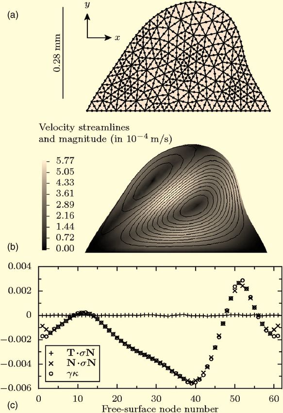
103303-2     Schindler, Talkner, and Hänggi                                                             Phys. Fluids 18, 103303 共2006兲

mented in the commercially available fluid-dynamics pro-             reference for this formulation can be found in the works of
gram FLUENT using a volume-of-fluid discretization. For a            Aris26 and Scriven,27 where the fluidic flow inside a curved
macroscopic system, this method worked fine. The method,             free surface is described.
however, fails if the system is scaled down to the microflu-              Recently, algorithms have been published that describe
idic parameter regime. In a simple test example, we found            time-dependent free-surface flows, even in three
that approximation errors of the free-surface boundary con-          dimensions.28–30 In these works, the free surface is moved
dition contributed to the force balance in the Navier-Stokes         mainly due to the kinematic boundary condition, i.e., it is
equations and were amplified in an uncontrolled manner.              advected passively. Concerning convergence, there has been
This typically gave rise to a spurious velocity field. It even       a controversy if the kinematic or rather the normal stress
occurred when we started the iteration with the known                boundary condition should be used to move the free surface.
solution. Problems with this method have also been reported          This issue was resolved by Silliman and Scriven, who state
by Renardy and Renardy16 and by Popinet and Zaleski.17               that for capillary numbers below unity, the normal stress it-
Lafaurie et al.18 find the spurious velocities to be of the order    eration converges well while a kinematic iteration eventually
surface-tension/viscosity, which is the dominant velocity            fails.22 In addition, when the kinematic boundary condition is
scale for microfluidic systems. Thus, the existing continuum         used for updating the free surface, the balance of normal
method appears to be inappropriate for the microfluidic pa-          stress that carries the effects of surface tension is not strictly
rameter regime.                                                      imposed. It is used when implementing the weak form of the
     Another approach of the first kind has recently been pro-       Navier-Stokes equations: In this context, an integration by
posed by Smolianski.19 He uses finite elements and a level-          parts yields an integral of the normal stress over the free
set description for the free surface and calculates curvatures       surface, which is then replaced by the corresponding surface
by derivatives of the distance function. He too encounters           integral of the tension forces. Similar techniques are com-
spurious velocity fields proportional to the ratio surface-          monly used for problems with outflow boundary conditions
tension/viscosity.                                                   or for Poisson’s equation with Neumann boundary condi-
     Methods of the second kind, representing the free sur-          tions. The correctness of the technique has been justified for
face by a sharp interface, are expected to work better in the        the outflow problem by Renardy.31 However, it is not evident
microfluidic parameter regime. Algorithms in this class are          whether it also works in the case in which the surface-tension
often referred to as “moving mesh” or “ALE” methods and              terms dominate the whole problem. The question remains in
generally require more involved techniques, keeping the              which sense the boundary condition is satisfied. Therefore,
computational mesh feasible and not too distorted.                   we found it necessary in our examples to visualize the terms
     A technique of the second kind that has successfully            involved in the free-surface boundary condition, thus prov-
been employed for tension-dominated free-surface problems            ing that they are correctly balanced.
is the boundary-element method.20,21 Pinch-off effects and                An important result of our variational description of the
droplet formations can be described by this method.14 The            tension terms is an improvement of the Newton algorithm
dimensionality of the equations is reduced to the dimension-         controlling possible mesh distortions at the free surface.
ality of the surface, which provides the basis for an efficient      Many algorithms implementing the weak form of the capil-
implementation. Unfortunately, this reduction can only be            lary boundary condition encounter intrinsic instabilities of
performed for Stokes equations with conservative body                the boundary mesh when significant changes of the free sur-
forces, which can be absorbed into the pressure term. In the         face take place. For the program surface evolver,32 this mani-
present investigation, we allow for nonconservative body             fests itself in shrinking and growing surface facets. Similar
forces that are of particular experimental relevance.9,10            effects have been observed by Brinkmann33 and Bänsch.28
     Pioneering works for the finite-element implementation          Our formulation of the capillary free surface is such that the
of the full free-surface problem were published by Scriven           free surface smoothly changes to the behavior of a rubber
and co-workers.22,23 They used spines to parametrize the             blanket when the boundary mesh becomes distorted. This
movements of the computational mesh in coating flow and              leads to an automatic regularization of the mesh without the
implemented Newton’s method for a Galerkin approximation             need of explicit remeshing or smoothing.
scheme. This work was later continued under the designation               In Sec. II, the mathematical formulation of the problem
“total linearization method” by Cuvelier and co-workers.24,25        is presented in terms of differential equations, together with
Their description requires a height function for the free-           the boundary conditions and the relevant parameter regime.
surface position, which makes it necessary to use well-              In Sec. III, we then reestablish the bulk equations and their
adapted coordinate systems. Whether a free surface will              boundary conditions by variational techniques. For the free
overhang must be known in advance.                                   surface, we introduce a differential-geometric notation that
     In the present paper, we extend the works of Scriven and        allows us to write the boundary condition in a weak form.
Cuvelier to arbitrary surface geometries. In our description,        Up to this point, a continuous description is used. Section IV
the parametrization of the free surface is given directly by         introduces the discretization of the problem by the computa-
the finite-element boundary parametrization. Thus, neither           tional mesh. The formulation of the tension forces as the
spines nor a height function are needed. To properly account         concurrent minimization of the free-surface area of single
for intrinsic curvatures of the free surface, all equations are      finite elements is a necessary requirement for the mentioned
formulated in a fully covariant form that allows for all             automatic regularization mechanism. Section V provides a
differential-geometric properties of the surface. An excellent       short summary of the whole algorithm. In Sec. VI, we

Downloaded 19 Oct 2006 to 193.174.246.34. Redistribution subject to AIP license or copyright, see http://pof.aip.org/pof/copyright.jsp
103303-3 Computing stationary free-surface shapes in microfluidics Phys. Fluids 18, 103303 共2006兲
present examples that show the accuracy of the algorithm Equations 共1兲–共6兲 have been simplified by assuming that
and two further examples for different values of the capillary at the free surface the fluid always stays in contact with a
and Bond numbers. Mathematical and algorithmic details are medium of low viscosity such as in the case of a water-air
deferred to Appendixes A–D. interface. Therefore, the viscous stress contribution of the air
does not show up in the balance equation 共6兲. We further
II. STATEMENT OF THE PROBLEM assume that the ambient pressure p0 is constant. Since the
pressure is determined by the Stokes equations only up to a
Throughout the paper, we use tensor notation in arbitrary
constant, we can split it into a part p1 with vanishing average
curvilinear coordinates. This will considerably simplify the
and use the ambient pressure p0 as an offset parameter that
differential geometric notation in the following sections. For
enters only in the normal stress balance 共6兲,
the formulation of the full Navier-Stokes equations in curvi-
linear coordinates, we refer to Aris.26 Repeated indices in co-
and contravariant positions are summed over. Indices pre-
ceded by a comma denote covariant derivatives, and gij is the
p共x兲 = p0 + p1共x兲 with 冕 V
p1dV = 0. 共7兲
metric tensor of the underlying coordinate system.
B. The parameter regime
A. The basic equations
By transforming both the bulk equation 共2兲 and the free
We study incompressible and stationary flows, which are boundary condition 共6兲 into dimensionless form employing
characterized by a small Reynolds number Re= x̄v̄ / . Here, viscosity scaling, one observes that the system may be char-
is the density of the fluid, its viscosity, and x̄ and v̄ acterized by two relevant ratios of forces, given by the di-
denote typical magnitudes of length and velocity. Under mensionless numbers
these conditions, the pressure field p and the velocity field
with components vi satisfy the Stokes equations,34 f̄ 共c兲x̄2 v̄
Bo = and Ca = . 共8兲
vi,i = 0, 共1兲 ␥ ␥
0 = ij,j + f i where 共2兲 Here, x̄, v̄, and f̄ 共c兲 denote typical magnitudes of length, ve-
locity, and the conservative part of the force density, respec-
ij = − pgij + 2eij, and eij = 共vi,j + v j,i兲/2, 共3兲 tively. Bo is a generalization of the Bond number, which is
and where ij is the fluidic stress tensor, eij the rate-of-strain usually defined in terms of gravitational forces only. The
tensor, and f i an external body force causing nontrivial capillary number Ca measures the viscous contribution to the
streaming and pressure patterns within a domain V. It can be surface deformation. In a system with static boundaries and
i
split into a conservative part f 共c兲 , which can be displayed as vanishing Reynolds number, we can express the velocity
the gradient of a potential and a nonconservative part f 共nc兲 i scale by the typical magnitude f̄ 共nc兲 of the nonconservative
with vanishing divergence. The domain V may be bounded part of the driving force, namely v̄ = x̄2 f̄ 共nc兲 / . This yields an
by rigid walls and by free surfaces, as, e.g., a droplet sitting alternative definition of the capillary number similar to that
on a substrate. Equations 共1兲 and 共2兲 then are subject to of the Bond number,
boundary conditions at the different parts of the boundary
V: First, the flow has to meet the kinematic boundary con- f̄ 共nc兲x̄2
Ca = . 共9兲
dition, requiring that the normal projection of a stationary ␥
velocity field vanishes at the boundary, i.e.,
These two numbers reflect the different effects of the conser-
viNi = 0. 共4兲
vative and nonconservative parts of the driving. In this sense,
At immobile sticky walls, we use the no-slip boundary con- Ca also provides a measure for the spatial changes of the
dition, according to which the velocity vanishes also in the velocity field. For small Ca, the flow is slow and changes
tangential directions of the boundary, implying smoothly, whereas for large Ca it may exhibit drastic gradi-
ents.
viT␣i = 0 at the walls. 共5兲
We propose a numerical scheme for the parameter re-
Here, T␣i denotes the ith component of the tangential vector gime where both Ca and Bo are of order unity or less. Thus,
T␣ 共␣ = 1 , 2 for a two-dimensional surface兲. The remaining pressure gradients and viscous forces can deform the free
boundary is a free surface that dynamically adjusts its posi- surface significantly. The surface tension is large enough,
tion such that the stress balance holds, however, to keep the whole fluid domain together; a pinch-
off is excluded. The viscosity renders the velocity field
ijN j = ␥Ni on free surfaces, 共6兲
smooth over the whole fluid domain and prevents the exis-
with the surface tension ␥ and the curvature . Note that we tence of boundary layers. For the considered case of station-
have omitted a term proportional to the gradient of the sur- ary flows on resting substrates in stationary domains, the
face tension and thus exclude Marangoni effects. This sim- contact lines always stay pinned. A rolling or slipping droplet
plifies the following calculations but does not present a prin- would raise additional challenges regarding the stress near
cipal restriction of our description. the contact line that are beyond the scope of this paper.
Downloaded 19 Oct 2006 to 193.174.246.34. Redistribution subject to AIP license or copyright, see http://pof.aip.org/pof/copyright.jsp103303-4 Schindler, Talkner, and Hänggi Phys. Fluids 18, 103303 共2006兲
space coordinates is conveniently described by the surface
derivatives of the parametrization functions 共cf. Ref. 26,
p. 215兲, i.e.,
ti
t,i␣ = . 共13兲
␣
The D-dimensional contravariant space-vector, t,i␣, represents
the components of the ␣th tangential vector T␣ of the sur-
FIG. 1. A sketch of the coordinate system on a two-dimensional surface A,
face. At the same time, t,i␣ is a covariant surface-vector. The
embedded into the three-dimensional space. The surface coordinates are scalar products of these tangential vectors determine the
mapped from the reference domain E 共left兲 onto the surface A 共right兲 via the components of the surface metric tensor a␣,
parametrization vector t共兲.
a␣ = gijt,i␣t,j and a = det共a␣兲. 共14兲
III. CONTINUOUS DESCRIPTION OF THE PROBLEM The normal vector follows as the normalized cross product
of two tangential vectors,
In order to formulate the numerical treatment of the free-
surface boundary condition, we first explore the physical ori- Ni = 21 ijk␣t,j␣t,k , 共15兲
gins of the active forces. We will then express each of them
and the curvature is given as the trace of the tensor b␣ of
by the first variation of a functional. A modified Newton’s
the second fundamental form of the surface,
method requires us to calculate the second variation.
= a␣b␣ with 共16兲
A. Physical aspects of the free-surface boundary
condition: First variations b␣ = t,i␣Ni . 共17兲
The surface tension term ␥Ni in the boundary condition
Using the parametrization 共11兲 of the free surface, we dem-
共6兲 arises from the fact that an interface between two differ-
onstrate in Appendix B that the change of the free-energy
ent phases “costs” free energy.34 To find the optimal configu-
contribution F with respect to a variation of the surface po-
ration, the surface is continually probing positions in its
sitions ti is given by
vicinity in order to minimize its free energy. For the case of
an applied conservative force f i = −⌽,i the system is static
共vi = 0兲, and the free-surface boundary condition is equivalent ␦F关␦t兴 = 冕 A
␥t,jgija␣␦t,i␣dA. 共18兲
to a minimization of a free-energy expression. This calcula-
tion is performed in Appendix A. By an integration by parts, this expression can be cast into a
Due to its thermodynamic origin, the surface tension form containing the curvature term of the free-surface
term results from a first variation of a functional. This carries boundary condition 共6兲, i.e.,
冕
over to the dynamic case 共vi ⫽ 0兲 in which the boundary
condition 共6兲 must hold at any instant of time. The contribu- ␦F关␦t兴 = − ␥Ni␦tidA 共19兲
tion of the free surface A to the free energy is given by the A
integral of the surface tension ␥ over A,
共see Appendix C also for the case of varying surface ten-
F= 冕 A
␥dA, 共10兲
sion兲. In this way, the curvature term in Eq. 共19兲 that con-
tains second spatial derivatives is replaced by a product of
two terms, each containing a first derivative in Eq. 共18兲. Es-
where dA denotes the infinitesimal surface area. Any smooth pecially for numerical applications, it is much more favor-
surface in a D-dimensional space may be parametrized by able to work only with first derivatives. This trick has been
D − 1 surface coordinates ␣ 共␣ = 1 , . . . , D − 1兲, which deter- used in the literature in different contexts.21,32,35,36,28 Seen
mine the coordinates ti共␣兲 of points in D-dimensional space from a physical perspective, version 共18兲 of the equation is
on the surface. Both surface and space coordinates are illus- the more natural one. Here, one directly deduces that forces
trated in Fig. 1. In our numerical studies, we restrict our- pulling along the tangential direction attempt to minimize the
selves to D = 2. The general framework, however, remains facet area of the boundary. On the basis of single finite ele-
valid also for D = 3. The surface coordinates ␣ are taken ments, this perspective will be used below for stabilizing the
from the parameter set E 傺 RD−1. With running through E, computational mesh.
the whole free surface A is covered, The left-hand side of Eq. 共6兲, namely ijN j, is the normal
tiE: → R: 哫 ti共兲, 共11兲 fluidic stress at the boundary. We now recapitulate how this
term can be understood as the result of a variational prin-
A = 兵e共i兲ti共兲兩 苸 E其. 共12兲 ciple. In a stationary system with rigid immobile boundaries,
the variational principle, which is attributed to Helmholtz
Here, e共i兲 is the ith basis vector in space. Throughout the and Korteweg,37–40 states that the Stokes equations yield
paper, we will use Greek letters for surface indices and Latin those velocity and pressure fields that represent a stationary
ones for space indices. The connection between surface and point of the functional
Downloaded 19 Oct 2006 to 193.174.246.34. Redistribution subject to AIP license or copyright, see http://pof.aip.org/pof/copyright.jsp103303-5 Computing stationary free-surface shapes in microfluidics Phys. Fluids 18, 103303 共2006兲
P= 冕 V
PdV = 冕V
关共− pgij + eij兲vi,j − f ivi兴dV. 共20兲
with the boundary conditions 共4兲–共6兲. The latter depend on
the shape of V via the normal vector at the boundary. Both
parts of this problem cannot be processed independently.
Vice versa, from the vanishing first variation of P, In principle, two options exist to approach this combined
冕 冕
problem. The first one is to implement a single numerical
P system for both the flow variables p and vi together with the
␦ P关␦ p兴 = ␦ pdV = − vi,i␦ pdV, 共21兲
V p V geometric variables ti. We will not follow this direction but
rather consecutively solve two smaller systems, one for the
␦ P关␦v兴 = 冕冉
V
P
vi
␦vi +
P
vi,j
冊
␦vi,j dV 共22兲
flow variables, depending on the current domain V, and a
second one for the parametrization of the boundary. We have
chosen this approach because the problem is linear in the
冕
flow variables but highly nonlinear in the geometric vari-
= 共− f i␦vi + ij␦vi,j兲dV 共23兲 ables ti. The nonlinearity is caused by the appearance of the
V inverse surface metric a␣ and of the Jacobi determinant con-
tained in dA in Eq. 共18兲. Thus, solving the Stokes equations
=− 冕 V
共f i + ij,j 兲␦vidV + 冖 V
ijN j␦vidA, 共24兲
in the fluidic system, as we call it, will be a standard problem,
while the nonlinear search for the correct boundary shape
will be done in the geometric system. Both systems are
the Stokes equations follow by setting the bulk contributions solved consecutively:
to zero. The boundary integral in Eq. 共24兲 provides the flu- 共1兲 Choose an initial domain V.
idic stress contribution to the free-surface boundary condi- 共2兲 Until convergence, repeat the following steps:
tion.
At this point, we see that the two terms in the stress 共a兲 Solve the fluidic system within the domain V.
balance Eq. 共6兲 have different physical origins. The surface 共b兲 Solve the geometric system using fixed values for
tension is of thermodynamic 共or rather of “thermostatic”兲 the pressure and velocity variables. This results in
nature while the fluidic stress stems from dynamic consider- an updated domain V.
ations. The first minimizes a free energy, while the second
minimizes a power. Formally, this difference is expressed by In three-dimensional space, Eqs. 共4兲–共6兲 pose four
the distinct variations ␦vi and ␦ti in the expressions ijN j␦vi boundary conditions. There are one too many for the linear
in Eq. 共24兲 and ␥Ni␦ti in Eq. 共19兲. Already for dimension- fluidic system to be fully determined. One boundary condi-
ality reasons they cannot be equal, nor can the functionals F tion is thus used for updating the parametrization of the free
and P be directly combined into a single variational prin- surface.24 The main challenge is the proper assignment of
ciple. specific boundary conditions for the two systems in order to
From an algorithmic point of view, a choice has to be make them solvable, uniquely determined, and robust. It is
made whether the free-surface boundary condition is ap- clear that the no-slip boundary condition 共5兲 at sticky walls
proximated by means of either ␦vi or ␦ti as test functions. In applies only to the fluidic system. The free-surface boundary
the Galerkin implementation of the problem, we will use the condition needs further consideration.
ansatz functions of the finite elements as test functions. In Here, again, a physical argument helps to choose the
order to acquire a consistent numerical algorithm, in this proper boundary condition. Either the stress by the fluid or
case both the velocity and the geometry parametrization its velocity is employed for moving the free surface. Accord-
must be approximated by ansatz functions of the very same ingly, either the normal stress balance 共6兲 or the kinematic
order. This is the first central result of the present work. boundary condition 共4兲 leads to an update of the surface in
It was stated by Bänsch28 共p. 42, cf. also citations 49 and the geometric system 共see the discussion by Saito and
50 therein兲 that a second-order approximation of the surface Scriven22 and our remarks in the Introduction兲. We choose
parametrization yields a “good discrete curvature,” whereas a our approach according to the following principle: The flu-
first-order one does not. The same can be seen below in Fig. idic system should be well defined as a stationary system
2. We are now able to substantiate Bänsch’s numerical ob- even if the boundary is fixed and is not part of the problem.
servation with the underlying physical mechanism. The ar- The kinematic boundary condition must then apply to the
gument is similar to that for the celebrated Ladyzhenskaya- velocity field to prevent the fluid from passing through the
Babuska-Brezzi requirement that velocity gradients have to free surface. Thus, the kinematic boundary condition cannot
be approximated by the same order as the pressure. From a be used for updating the surface.
physical perspective, this is not astonishing, because both are Before the correct boundary shape is reached, the vis-
components of the stress tensor. cous stress of the flow may force the free surface into an
arbitrary direction. By its very nature, however, the tension
B. Splitting the problem into two numerical systems
force always stays normal on the free surface. Only normal
For free boundaries, a twofold problem must be solved: forces can be compensated by a free surface. As a conse-
共i兲 The unknown fluid domain V has to be determined and quence, the tangential projection of the normal stress has to
共ii兲 the Stokes equations 共1兲 and 共2兲 have to be solved in V, vanish.41 In the proposed scheme with two separated sys-
Downloaded 19 Oct 2006 to 193.174.246.34. Redistribution subject to AIP license or copyright, see http://pof.aip.org/pof/copyright.jsp103303-6 Schindler, Talkner, and Hänggi Phys. Fluids 18, 103303 共2006兲
tems, it is the fluidic system that must ensure the tangential The first two integrals on the right-hand side contain the
components of the free boundary condition 共6兲, i.e., changes of the normal vector 共15兲 and the infinitesimal sur-
face area dA = 冑ad due to changes of the boundary shape.
共vi,j + v j,i兲Nit,j␣ = 0 for all ␣ . 共25兲
Both can be calculated along the lines of Appendix B. The
As in Eq. 共6兲, the surface tension ␥ has been set constant. For third integral expresses the change of the fluidic stress ij on
the velocity variables, this constitutes a perfect-slip boundary the boundary caused by changes of its position. The shape
condition, which resembles a Neumann boundary condition. changes act on the velocity field via the boundary conditions
We thus find the fluidic system to be fully determined and 共4兲 and 共25兲 of the Stokes equations. Unfortunately, this in-
physically well defined even for fixed boundaries by the con- direct response of the viscous stress tensor to the changes of
ditions 共4兲, 共5兲, and 共25兲. shape cannot be expressed explicitly. We therefore assume
The geometric system is then responsible for the remain- that this dependence is weak. The boundary conditions affect
ing normal component of the stress balance 共6兲, only the velocity field, not the pressure, which is determined
only by the applied external force. A Taylor expansion of the
− p + 共vi,j + v j,i兲NiN j = ␥ , 共26兲
pressure field around the free surface yields for the change of
which is used as the update equation for the boundary. A the stress tensor,
given trial position of the free surface is updated if Eq. 共26兲 ␦ij关␦t兴 ⬇ − gij p,k␦tk . 共30兲
is violated.
This approximation assumes that the fluidic and the geomet-
C. Second variation with respect to the surface ric systems are decoupled to the extent that the viscous part
parametrization of the stress tensor in the vicinity of the boundary is not
affected by small boundary changes. Note that this assump-
In a first implementation we used a direct and explicit
tion influences only the rate of convergence but not the final
update algorithm moving the boundary into a normal direc-
result. The difficulty to describe the mutual dependence of
tion with a step width that is determined by a parameter
velocity field and surface geometry is not a consequence of
and the residual of Eq. 共26兲. The discretization of this update
splitting the problem into two separate systems, but a general
can be found below in Eq. 共54兲. Depending on the value of ,
problem that applies equally to the combined approach. Al-
this method exhibited strong instabilities. Although advanced
together, the right-hand side of Eq. 共29兲 becomes approxi-
techniques for determining an apt value for seem to exist
mately
共cf. the program Surface Evolver by Brakke32兲, we prefer a
modified Newton-Raphson iterative method. This has the ad-
vantages of faster convergence and less strong dependence 冕 A
兵共␦tiijN j兲共␦t,k␣gkla␣t,l兲 − 共␦tiijt,j␣兲a␣共␦t,kNk兲
on . It requires an additional variation of the surface free
energy for the assembly of the geometric system. Using the − ␦tiNi p,k␦tk其dA. 共31兲
same calculus as in Appendix B, we find the second variation
of the free-energy contribution F of a one-dimensional free
surface, IV. DISCRETIZATION OF THE PROBLEM
␦2F关␦t, ␦t兴 = ␦ 冉冕 A
␥gija␣t,j␦t,i␣dA 冊 共27兲 We propose a discretization of the above equations by
means of a Galerkin approximation scheme that is known to
work well for minimization problems. As variables we intro-
= 冕
A
␥␦t,i␣␦t,j共NiN ja␣ + ti␣tj − tit␣j 兲dA, 共28兲
duce the velocity components u and v in the x and y direc-
tion, respectively, the pressure p, and additional variables r
and s for the coordinates of the boundary parametrization
where the contravariant surface indices are introduced in vector t. The continuous fields are discretized using ansatz
Appendix B. Note that the precise form of the second varia- functions, weighted with the corresponding degrees of free-
tion influences only the convergence of the iteration, but not dom 共DoF兲,
the solution, which solely depends on the first variation.
u共x兲 = 兺 udd共x兲, v共x兲 = 兺d vdd共x兲, 共32兲
Also the flow velocity, and by this the viscous stress, d
depends on the shape of the surface. The formulation of the
p共x兲 = 兺 pdd共x兲,
modified Newton method requires also the change of the
共33兲
fluidic stress integral due to changes of the free boundary,
冉冕 冊 冕
d
␦ ijN j␦tidA 关␦t兴 = ␦tiij␦N j关␦t兴dA r共x兲 = 兺 rdd共x兲, s共x兲 = 兺 sdd共x兲, 共34兲
A A
d d
+ 冕 E
␦tiijN j␦冑a关␦t兴d where the sum runs over all DoFs. The fluid velocity com-
ponents u , v are approximated by the second-order finite
冕
elements 共FEs兲 and the pressure variable p by first-order
+ ␦ti␦ij关␦t兴N jdA. 共29兲 FEs . For the position variables r , s we predominantly used
A second-order FEs, but for accuracy and other testing reasons
Downloaded 19 Oct 2006 to 193.174.246.34. Redistribution subject to AIP license or copyright, see http://pof.aip.org/pof/copyright.jsp103303-7 Computing stationary free-surface shapes in microfluidics Phys. Fluids 18, 103303 共2006兲
we also tried first-order FEs. We denote the position FEs
with . All FEs are of the Lagrange family,6 having ansatz
ud = wd + 兺 wdeue ,
e⫽d
共44兲
functions that are 1 at exactly one node of the mesh and 0 at
all others. The DoFs are then equal to the function values at which represent the boundary condition in question. The
the nodes. This property is most convenient for the position DoF ud is then completely eliminated from the linear system
variables 共rd , sd兲 that coincide with the coordinates of the 共35兲. By such constraint equations we write the kinematic
node d. boundary condition 共4兲 as
A. The fluidic system
0 = 兺 共ueNx + veNy兲e , 共45兲
The fluidic system is formulated in a standard way. e
Equation 共2兲 is tested with the second-order FEs , while the
continuity equation 共1兲 is tested with the first-order FEs . the no-slip condition at the walls
The system consists of the following linear equations for the
DoFs, which are collected in the vectors uជ , vជ , pជ with compo-
nents ud , vd , pd, respectively, 0 = 兺 共ueTx + veTy兲e , 共46兲
e
冢 冣冢 冣 冢 冣
Kuu 0 Kup uជ Lu
0 Kvv Kvp vជ = Lv 共35兲 and a weak version of the tangential projection of the free-
surface boundary condition 共25兲,
K pu K pv 0 pជ 0
with the entry matrices K and entry vectors L given by
0=兺 冉 冊冉
ue 2TxNx T xN y + T y N x
冊
冕 冖
·
e ve T xN y + T y N x 2TyNy
关Kuu兴de = d · edV − dN · edA, 共36兲
V V
⫻ 冕 冉 冊d
x e
ye
dA. 共47兲
冕 冖
V
关Kvv兴de = d · edV − dN · edA, 共37兲
V V The constraint equations differ only in the values of wde. The
inhomogeneity wd is zero in all three equations. Nonzero
关Kup兴de = − 冕 V
共xd兲edV + 冖V
deNxdA, 共38兲
inhomogeneities would result in the presence of gradients of
the surface tension or in the case of tangentially moving rigid
boundaries.
冕 冖
For the boundary condition 共47兲, which is equivalent to a
关Kvp兴de = − 共yd兲edV + deNydA, 共39兲 perfect-slip condition, an improper choice of the normal di-
V V rection can cause spurious contributions to the velocity field
共see Behr,42 Walkley et al.,43 and our remarks stated in the
关K pu兴de = − 冕 V
dxedV, 共40兲
Introduction兲. In the presence of conservative forces only, we
did not find such spurious flows in our results.
The fact that the free boundary condition 共47兲 cross-links
冕
all DoFs residing at boundary nodes presents a serious prob-
关K pv兴de = − dyedV, 共41兲 lem. Each of the DoFs is in principle linked to all its neigh-
V bors on the boundary. This leads to a nearly filled system
matrix that is unfavorable regarding memory capacity and
关Lu兴d = 冕V
d f xdV, 共42兲
computing time. We found that an iterative method can over-
come this problem. Instead of cross-linking a boundary DoF
with all its neighbors, for some of them we take their old
冕
values, as is detailed in Appendix D. After some iterations,
关Lv兴d = d f ydV. 共43兲 the full boundary condition 共47兲 is established. The draw-
V back of this scheme is that the constraint equations have
to be reassembled after every solution step of the fluidic
All integrals are assembled in a loop over the elements and
system.
the sides of the mesh, using a fifth-order Gaussian quadrature
rule. The fluidic system could likewise implement the sta-
B. The geometric system
tionary Navier-Stokes equations with a small Reynolds num-
ber; we choose the Stokes equation for simplicity reasons In the geometric system, a modified Newton method is
here. employed to perform the nonlinear search for the correct
The boundary conditions are imposed by a constraints boundary position. This scheme corresponds to a minimiza-
technique for the matrix and for the right-hand side in Eq. tion of the free energy F, while taking the fluidic stress into
共35兲. A constrained DoF ud is expressed by an inhomogeneity account. The boundary update equation can be written in a
plus a weighted sum of other DoFs, discretized form as
Downloaded 19 Oct 2006 to 193.174.246.34. Redistribution subject to AIP license or copyright, see http://pof.aip.org/pof/copyright.jsp103303-8 Schindler, Talkner, and Hänggi Phys. Fluids 18, 103303 共2006兲
0 = 关Lr兴d共rជ,sជ,uជ , vជ ,pជ 兲 ª
F
rd
+ 冕A
dxjN jdA,
sides cause badly conditioned matrices and make the algo-
rithm unstable. Several algorithms implementing the weak
form of the free-surface boundary condition encounter these
共48兲
冕
intrinsic instabilities of the boundary mesh. For the program
F Surface Evolver this manifests itself in shrinking and grow-
0 = 关Ls兴d共rជ,sជ,uជ , vជ ,pជ 兲 ª + dyjN jdA,
sd A ing surface facets. It is therefore recommended to monitor
the mesh quality and remove too small or split too large
where d enumerates the geometric variables, and L and F are elements.32 Similar effects were reported by Brinkmann.33
functions of the arrays rជ , sជ, etc. containing the DoFs. For the In Sec. III B, the assignment of the boundary conditions
original Newton-Raphson method, the geometric system re- to the fluidic and the geometric systems was described.
peatedly has to solve the linear system of equations44 There, we found that the presence of incompatible forces
冉 关Lr兴d/re 关Lr兴d/se
关Ls兴d/re 关Ls兴d/se
冊 冉
共old兲
rជ共new兲
e
sជ共new兲
e
− rជ共old兲
e
− sជ共old兲
e
冊 may easily destroy a free surface that essentially attempts to
minimize the lengths A共m兲 of the free-surface sides in each
element m. Because all fluidic stresses are constrained to
=− 冉 冊
关Lr兴d
关Ls兴d
共old兲
, 共49兲
have only normal components, we are free to use additional
tangential force components for keeping the boundary mesh
as regular as possible. This can be done during the assembly
where 苸 关0 , 1兴 is a step-size parameter. In the original of the system matrices by weighting the surface tension by
Newton method, the block matrices on the left-hand side of the element side length A共m兲, divided by the average length
Eq. 共49兲 consist of the second variations given by Eq. 共28兲. 具A共m兲典 of all element sides contributing to the free surface. Of
This method turns out to be numerically unstable. This is a course, this weighting factor becomes ineffective if all sides
surprising fact, because the calculation that has led to Eq. have equal length. Any length difference of adjacent sides
共28兲 consists of two straightforward variations. A convergent causes an additional force that tries to equalize them. The
algorithm is obtained by modifying the block matrices, rep- tension forces for each element side are then equivalent to a
resenting instead of Eq. 共28兲 the integral first variation of the functional ␥A共m兲
2
/ 共2具A共m兲典兲, which de-
冕 A
␥␦t,i␣␦t,jgija␣dA. 共50兲
scribes a rubber band with Hookean forces. Instead of ␦F关␦t兴
from Eq. 共18兲, we thus assemble on each element
␥ A共m兲
The only fixed points of the Newton-Raphson method 共49兲 ␦共A共m兲
2
兲关␦t兴 = ␥ ␦A共m兲关␦t兴. 共51兲
2具A共m兲典 具A共m兲典
are the zeros of the vector 共Lr , Ls兲. These are independent of
2
the particular choice of the matrix on the left-hand side of The second variations of A共m兲 and A共m兲 / 2 are not proportional
Eq. 共49兲. The modified matrix leads to a convergent iteration to each other,
toward the accurate solution. This is confirmed by the ex-
amples in Sec. VI B. The analogous argument applies to the ␥ A共m兲 2
␦2共A共m兲
2
兲关␦t, ␦t兴 = ␥ ␦ A共m兲关␦t, ␦t兴
approximation in Eq. 共30兲. 2具A共m兲典 具A共m兲典
The search for the correct boundary shape is strongly
1
nonlinear in the position variables. In order to remove the +␥ 共␦A共m兲关␦t兴兲2 . 共52兲
main nonlinearities, which are caused by the surface metric 具A共m兲典
expressions 冑a and a␣, the nodes of the elements are moved In the implementation we therefore took only the first term
to their corresponding coordinates 共rd , sd兲 after each step of on the right-hand side of Eq. 共52兲. In this sense, we did not
the geometric system. Then, all integrals can be performed strictly implement the behavior of a rubber band, but yet a
directly on the element edges. Also the normal vector can be stabilized version of the free-surface tension terms. After
taken from the element sides. In the previous section, we convergence, all boundary sides of the mesh representing the
used a convenient variational notation to express the change free surface have equal lengths, and the extra terms
of the free-energy contribution F by changes of the boundary A共m兲 / 具A共m兲典 do not change the behavior of the free surface.
parametrization. Essentially the same equations are obtained
by differentiating the discrete version of F with respect to the
DoFs, which are the nodal degrees of freedom of the corre- V. SUMMARY OF THE ALGORITHM
sponding variables. The only difference is that the variation Here, we provide a short overview of the complete algo-
␦ti in the continuous formulation must be replaced by the rithm. The required steps are as follows:
vectorial test function dei, and the variation ␦t,i␣ by its tan-
gential derivative T␣ · dei. 共1兲 Choose an initial mesh and initial ambient pressure p0.
共2兲 Until convergence, repeat the following steps:
C. Controlling the tangential displacements
共a兲 Smooth the inner mesh if it is too distorted.
of boundary nodes
共b兲 Repeatedly solve the fluidic system for p, u, and v
For a given discretization, we must not only find the until the perfect-slip boundary condition is estab-
correct boundary shape, but its discretization should also re- lished.
main well-proportionate. Very long and very short element 共c兲 Subtract the average from p.
Downloaded 19 Oct 2006 to 193.174.246.34. Redistribution subject to AIP license or copyright, see http://pof.aip.org/pof/copyright.jsp103303-9 Computing stationary free-surface shapes in microfluidics Phys. Fluids 18, 103303 共2006兲
共d兲 Solve the geometric system for the new boundary. summarize also the terms of the geometric system. The up-
At the same time, search for the value of p0 that date Eq. 共49兲 is written as
keeps the volume unchanged.
共e兲 Set the mesh boundary nodes to the parametrization
values of the geometric system. 冉 Krr Krs
Ksr Kss
冊冉 冊 冉 冊 冉
rជ共new兲
sជ 共new兲
=−
Lr
Ls
+
Krr Krs
Ksr Kss
冊冉 冊rជ共old兲
sជ共old兲
The fluidic system is assembled according to Eqs. 共53兲
共35兲–共43兲 with constraints that account for the proper bound-
ary conditions. To give the full algorithm at this point, we with entries that are assembled per element m,
关Lr共m兲兴d = 冕
A共m兲
d共ex · · N兲dA +
␥A共m兲
具A共m兲典
冕
A共m兲
共d · T兲共ex · T兲dA, 共54兲
共m兲
关Krr 兴de = − 冕
A共m兲
de共ex · p兲共ex · N兲dA + 冕 A共m兲
d共e · T兲兵共ex · N兲共ex · T兲 − 共ex · T兲共ex · N兲其dA +
␥A共m兲
具A共m兲典
冕
A共m兲
共d · T兲
⫻共e · T兲dA, 共55兲
共m兲
关Krs 兴de = − 冕
A共m兲
de共ex · p兲共ey · N兲dA + 冕 A共m兲
d共e · T兲兵共ex · N兲共ey · T兲 − 共ex · T兲共ey · N兲其dA. 共56兲
The remaining entries can be obtained by permutations of x few iteration steps, starting from the exact solution, the
and y together with r and s. Again, constraints were used to finite-element approximation was completely destroyed. Us-
keep the contact lines pinned. In all applications we used ing second-order FEs, the instability was similar.
values of between 0.1 and 1.0.
B. Testing the accuracy of the modified Newton
algorithm
VI. NUMERICAL EXPERIMENTS
In order to confirm the accuracy of the curvature ap-
We performed all our test cases for a two-dimensional proximation of the algorithm in Eqs. 共53兲–共56兲, we test two
fluid. The programs were written using the open-source cases that can be solved analytically. Similar to the calcula-
C⫹⫹ library libmesh,45 which allows changes to the element tion in Appendix A, a prescribed pressure determines the
geometry in a user’s routine and provides a powerful con- free-surface shape. Then, the approximation in Eq. 共30兲 be-
straint method. comes exact and simplifies to
A. The instability of a “direct explicit update” ␦ij = − gij p,k␦tk . 共58兲
algorithm
Thus, possible approximation errors result only from the dis-
In a first numerical example, we did not use the modified cretization of the curvature.
Newton’s method with the update rule 共53兲, but instead with Figure 2共a兲 depicts the most simple situation in which a
the direct and explicit update rule homogeneous pressure field deforms the boundary into a cir-
冉 冊 冉冊冉 冊
rជ共new兲
sជ共new兲
= −
Lr
Ls
+
rជ共old兲
sជ共old兲
. 共57兲
cular arc, as in the previous example. The free surface shape
is approximated by the sides of five second-order FEs and 14
first-order FEs, respectively. In dimensionless units, the sur-
The stability of this update rule sensibly depends on the step- face tension is ␥ = 1 and the prescribed pressure p0 = 2 pro-
size parameter . The allowed range of is a function of the duces a circle with radius R = 1 / 2 as the exact solution. The
size of the elements, the curvature, etc. In a simple situation, initial geometry of both surface approximations was the
a homogeneous pressure field deforms the boundary into a straight connection between the fixed end points. Good con-
circular arc with radius R = −1 / = p0 / ␥. For the combination vergence was reached after 100 iterations with step-size pa-
R = 0.5, ␥ = 1, and p0 = 2, we found the update rule 共57兲 to be rameter = 1. The comparison of a second-order approxima-
stable for 14 first-order FEs and a given step size = 0.05. tion with a first-order one, using more than twice as many
The resulting approximation is indistinguishable from the FEs, clearly reveals the superiority of the second-order pa-
first-order approximation in Fig. 2. In contrast, the update is rametrization. The relative errors of the numerically resulting
unstable for the same step size and 52 first-order FEs. After a curvatures are about 8.6⫻ 10−6 and 5.0⫻ 10−3 for the
Downloaded 19 Oct 2006 to 193.174.246.34. Redistribution subject to AIP license or copyright, see http://pof.aip.org/pof/copyright.jsp103303-10 Schindler, Talkner, and Hänggi Phys. Fluids 18, 103303 共2006兲
FIG. 2. Panel 共a兲 depicts the free-surface deformation, which is caused by a
prescribed homogeneous pressure p0 = 2. The exact solution 共dashed curve兲 FIG. 3. Same as Fig. 2, for an expected sinusoidal boundary shape
in Cartesian coordinates x and y is a half-circle with radius 1 / 2. Two finite- y = h共x兲 = 0.25 sin共4x兲, generated by the prescribed pressure of Eq. 共59兲
element approximations are presented, one with five second-order FEs 共up- with surface tension ␥ = 1. The approximated free surface consists of 40
per solid curve兲 and another one with 14 first-order FEs 共lower solid curve兲. second-order FEs.
The first-order FEs are bounded by vertices 共indicated by small circles兲,
while the second-order FEs also contain second-order nodes 共small crosses兲
in between. Panel 共b兲 compares an estimate of the Laplace pressure ␥ and
the applied pressure p0 as a function of the spatial x coordinate. The agree-
␣2 sin共x兲
ment is excellent, except for the outliers near the end points, where the p共x,y兲 = − ␥共x兲 = ␥ . 共59兲
estimate of the curvature is less accurate. 关1 + ␣22 cos2共x兲兴3/2
Again, the approximation in Eq. 共30兲 becomes exact, and we
second-order and first-order approximations, respectively. expect similar discretization errors as in the previous ex-
These values are obtained from the position of the topmost ample. The initial geometry was the straight line between the
node. end points of the surface. Good convergence was reached
The result of an alternative estimate of the approxima- after 60 iterations with step size = 1. The relative error of
tion error is visualized in Fig. 2共b兲. The normal vectors at the curvature 6.7⫻ 10−3 is larger than in the previous ex-
each node are calculated from the resulting finite-element ample because the parts with the maximal curvature are dis-
side. Due to the elements being second-order, we obtain a cretized less densely. Nevertheless, the error is still small
unique normal vector at second-order nodes. At vertices enough to reproduce the expected boundary shape with ex-
where two elements meet and where the surface parameter- cellent accuracy. It decreases with the number of approxi-
ization is not smooth, we average the resulting two normal mating elements. A first-order approximation leads to a much
vectors. The curvature estimate at a node in Fig. 2共b兲 is then larger, possibly intolerable error of 2.0⫻ 10−1. The side
given by the curvature of a circle sector that is determined by lengths of the elements in Fig. 3共a兲 vary only by ±0.007%.
the two neighbors of the specific node. The sector is bounded This small deviation demonstrates that the mesh regulariza-
by the two corresponding normal vectors; its chord length tion method does not influence the final behavior of the free
equals the distance between the two neighbors. This yields a boundary.
reconstruction of the curvature from the change of the nor- Concerning the discretization errors of the curvature, the
mal vector per arclength of the surface. It is clear by con- accuracy test in Fig. 3 covers already the general case. Ac-
struction that the normal vector at the end points cannot be cording to the construction of the algorithm, the flow exerts
reliably estimated. This causes the outliers in Fig. 2共b兲. All stress on the boundary only in a normal direction. Whether
other nodes fit well. this stress is of viscous nature or due to a pressure difference
In the next accuracy test, depicted in Fig. 3, a variable is irrelevant for the resulting curvature.
pressure is prescribed, for which the resulting boundary
C. A deformed microdroplet
shape is known. Figure 3共a兲 illustrates the approximation of
a sinusoidal boundary height function y = h共x兲 = ␣ sin共x兲, In order to explicitly show that the quality of the curva-
which is caused by the corresponding pressure field ture discretization does not depend on the origin of the ap-
Downloaded 19 Oct 2006 to 193.174.246.34. Redistribution subject to AIP license or copyright, see http://pof.aip.org/pof/copyright.jsp103303-11 Computing stationary free-surface shapes in microfluidics Phys. Fluids 18, 103303 共2006兲
FIG. 4. The force density that models the effect of the surface-acoustic
wave in the droplet given in Fig. 5. Panel 共a兲 depicts the nonconservative
part that causes the flow; 共b兲 shows the potential of the conservative part that
contributes only to the pressure.
plied normal stress, we return to the introductory motivation
for the present work. The previous examples were analyti-
cally solvable. The form and internal streaming of micro-
droplets, however, cannot be determined analytically.
In the experiment, the internal flow is agitated by a
surface-acoustic wave 共SAW兲 due to the acoustic streaming
effect.46 Because the very details of the impact of the SAW
are not known, we model it here by a body force that is
active in the fluid only, as depicted in Fig. 4. The force is
concentrated in a narrow channel that starts at the left contact
point where the SAW enters and continues into the fluid. The
fluid is carried along this channel, from the entry point of the
SAW into the droplet, giving rise also to a back flow.47 Ad-
ditionally, the force has a strong conservative portion that is
balanced by the pressure in the fluid.
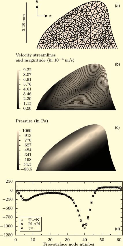
FIG. 5. A deformed microdroplet, sitting on a flat substrate with pinned
The resulting stationary droplet shape and the internal contact points. The deformation is due to an internal pressure and viscous
velocity and pressure fields are presented in Fig. 5. The ini- flow, both caused by the body force density illustrated in Fig. 4. The mate-
tial shape was a half-circle with the same two-dimensional rial properties are those of water surrounded by air at room temperature. The
volume. Good convergence was reached after seven itera- panels depict the computational grid 共a兲, the flow 共b兲, and the pressure field
共c兲, respectively. Note that the deformation is predominantly caused by the
tions with a step-size parameter = 0.5. The material proper- pressure, which corresponds to the case in which CaⰆ Bo. In panel 共d兲, the
ties are those of water and air at room temperature, i.e., free-boundary condition is examined: The normal stress N · N equals the
= 10−3 kg/ ms and ␥ = 72.8⫻ 10−3 N / m. The deformed Laplace pressure ␥; the tangential stress T · N vanishes.
boundary consists of two regions, one with negative curva-
ture 共as the initial half circle兲 and another one at the right
flank of the droplet with positive curvature. The—admittedly the free surface is significantly deformed, its discretization
strange—deformation of the droplet qualitatively agrees with by finite-element sides is as regular as possible. Their lengths
the experimentally observed jumping droplet in Fig. 4 of the vary only by 4.5⫻ 10−5%. This guarantees that the behavior
publication by Wixforth et al..10 The deformation is due to of the boundary is indeed that of a free surface and is not
the large conservative contribution of the driving force and influenced by the automatic regularization technique de-
the resulting pressure. The viscous forces for the given ve- scribed in Sec. IV C. Figure 5共d兲 quantifies the normal stress
locities are far too weak to lead to a substantial deformation condition. For each node, we integrated the normal and the
of the free surface. The capillary number for the illustrated tangential component of the normal stress, weighted with the
flow is Ca⬇ 10−5; the Bond number is around 1. Although corresponding ansatz function of the node. The tangential
Downloaded 19 Oct 2006 to 193.174.246.34. Redistribution subject to AIP license or copyright, see http://pof.aip.org/pof/copyright.jsp103303-12 Schindler, Talkner, and Hänggi Phys. Fluids 18, 103303 共2006兲
the convergence rate of the modified Newton method, and
convergence was achieved after 30 iterations.
VII. SUMMARY AND OUTLOOK
In this work, we presented a weak formulation of free-
surface boundary problems in arbitrary coordinate systems.
The steps of the derivation are physically and mathemati-
cally founded using variational techniques for the Stokes
equations and the differential geometry of the surface. We
found that the applicability of different numerical treatments
of the curvature terms depends strongly on the scales of the
system. Our method is designed for Bond and capillary num-
bers assuming values from zero up to unity. Which one is
larger plays no role.
A decisive benefit of our method is the automatic control
of mesh regularity at a free surface. Many algorithms imple-
menting the weak form of the free-surface boundary condi-
tion encounter intrinsic instabilities of the boundary mesh.
Often, it is therefore necessary to create a completely new
mesh after several iteration steps. Our formulation includes a
smooth transition to the behavior of a rubber blanket when
the boundary mesh becomes distorted. This leads to an in-
herent regularization of the mesh without affecting the be-
havior of the free surface.
As another important result, we find that for physical
reasons the geometric variables for the parametrization of the
free surface should be approximated on the same level of
accuracy as the velocity variables. This substantiates numeri-
cal observations reported by Bänsch.28
FIG. 6. A microdroplet of similar shape as in Fig. 5, deformed only by the The quality of our numerical approach is tested by two
viscous stress at the boundary. The flow is driven by the nonconservative
analytically solvable examples. The numerical results for the
force density of Fig. 4共a兲 and vanishing conservative part of the force den-
sity. The surface tension ␥ is 105 times smaller than in Fig. 5. This corre- curvature of the free surface and for the stress that causes the
sponds to the case BoⰆ Ca. Panel 共c兲 corresponds to Fig. 5共d兲. deformation confirm that the free-surface boundary condition
is indeed satisfied in the implemented weak sense. Moreover,
transcending a weak-sense result, a reliable reconstruction of
the curvature by the normal vectors of the finite-element
component vanishes perfectly. The normal component coin- sides is feasible. Two further examples illustrate that the ratio
cides well with the reconstruction estimate of the curvature, of capillary number and Bond number has only a weak in-
which was described in the previous examples. Thus, the fluence on the stability of the algorithm.
free-surface boundary condition is indeed satisfied. The presented covariant formulation opens the possibil-
In order to prove that our algorithm can likewise pro- ity to utilize the powerful differential geometric description
duce stable results in the parameter regime BoⰆ Ca, we con- of free surfaces in finite-element implementations of the
sider a droplet that is deformed only by viscous stress. In Stokes equations. It thus provides a natural approach to treat
Fig. 6, we used the same nonconservative force that is visu- surfaces and interfaces with a richer behavior, such as lipid
alized in Fig. 4, but we omitted the conservative part. Thus, vesicles containing bending stiffness, area constraints, and
the pressure was constant and Bo= 0. With the same water- much more. Many potential applications can be found in the
air interface tension as in the previous example, the droplet literature on lipid vesicle geometry, where other expressions
would acquire an almost spherical shape. To obtain a com- for free-energy contributions of more complicated surfaces
parable deformation as in the previous case together with are in use.48–50
Ca⬇ 1, we took an artificial 105 times smaller surface ten- Extensions of the presented approach toward moving
sion. The initial geometry was the droplet shape of Fig. 5. In contact lines, time-dependent flows, and a three-dimensional
this example, the stress that deforms the free surface depends implementation are possible. There are still some hurdles to
much more strongly on the shape of the surface itself. Thus, be overcome that can be clearly seen in our derivation. One
the approximation in Eq. 共30兲, expressing surface-stress of them is the principally unknown mutual dependence of the
variations by variations of the surface shape, becomes ques- stress tensor and the surface parametrization, where we in-
tionable. As a result, we had to set the numerical parameter troduced the approximation 共30兲. Another one is the under-
to a smaller value than in the previous example, in order to standing of the numeric instabilities caused by the second
reduce the step size of the surface update. This deteriorates variation of the free energy of the surface, see Eqs. 共28兲 and
Downloaded 19 Oct 2006 to 193.174.246.34. Redistribution subject to AIP license or copyright, see http://pof.aip.org/pof/copyright.jspYou can also read