Construction of an Optimal Solution for a Real-World Routing-Scheduling
←
→
Page content transcription
If your browser does not render page correctly, please read the page content below
Construction of an Optimal Solution for a Real-World Routing-Scheduling-
                              Loading Problem
 Construcción de una Solución Óptima para un Problema de Asignación de Rutas, Horarios y
                                 Cargas del Mundo Real
         Juan Javier González Barbosa, José Francisco Delgado Orta, Héctor Joaquín Fraire Huacuja,
                     José Antonio Martínez Flores and María Lucila Morales Rodríguez

                                      Instituto Tecnológico de Ciudad Madero, México
{jjgonzalezbarbosa, francisco.delgado.orta}@gmail.com, hfraire@prodigy.net.mx,
                        {jose.mtz, lmorales}@gmail.com

                       Article received on July 20, 2009; accepted on November 14, 2009

       Abstract
       This work presents an exact method for the Routing-Loading-Scheduling Problem (RoSLoP). The objective of
       RoSLoP consists of optimizing the delivery process of bottled products in a company study case. RoSLoP,
       formulated through the well-known Vehicle Routing Problem (VRP), has been solved as a rich VRP variant
       through approximate methods. The exact method uses a linear transformation function, which allows the reduction
       of the complexity of the problem to an integer programming problem. The optimal solution to this method
       establishes metrics of performance for approximate methods, which reach an efficiency of 100% in distance
       traveled and 75% in vehicles used, objectives of VRP. The transformation function reduces the computation time
       from 55 to four seconds. These results demonstrate the advantages of the modeling mathematical to reduce the
       dimensionality of problems NP-hard, which permits to obtain an optimal solution of RoSLoP. This modeling can
       be applied to get optimal solutions for real-world problems.
       Keywords: Optimization, Routing–Scheduling–Loading Problem (RoSLoP), Vehicle Routing
       Problem (VRP), rich VRP.

       Resumen
       Éste trabajo presenta un método exacto para el problema de Asignación de Rutas, Horarios y Cargas (RoSLoP). El
       objetivo de RoSLoP consiste en optimizar el proceso de entrega de productos embotellados en una compañía caso
       de estudio. El problema RoSLoP, formulado a través del conocido Problema de Enrutado de Vehículos (VRP), ha
       sido resuelto como una variable VRP enriquecida a través de métodos aproximados. El método exacto usa una
       función de transformación lineal, la cual permite la reducción de la complejidad del problema a un problema de
       programación entera. La solución óptima para éste método establece las métricas del desempeño para los métodos
       aproximados, los cuales alcanzan una eficiencia del 100% en distancia recorrida y 75% en vehículos utilizados,
       objetivos del VRP. La función de transformación reduce el tiempo del cálculo de 55 a cuatro segundos. Éstos
       resultados demuestran las ventajas del modelado matemático para reducir la dimensionalidad de problemas NP-
       Duros, lo cual permite la obtención de una solución óptima del problema RoSLoP. Éste modelado puede ser
       aplicado para obtener las soluciones óptimas para problemas del mundo real.
       Palabras Clave: Optimización, Problema de Asignación de Rutas, Horarios y Cargas (RoSLoP),
       Problema de Enrutado de Vehículos (VRP), Problema VRP Enriquecido.

1 Introduction
The distribution and delivery processes are inherent to many manufacturing companies; in other cases, it is the main
function of several service businesses. Though this could be considered in consequential, however, merchandise
delivery in due time with the minimum quantity of resources, reduces operation costs, yielding savings between 5 to
20 % in total costs of products [Toth, P. and D. Vigo, 2001]. In recent years, many researchers have approached
transportation problems based on real situations in two ways: formulating rich models of solution and developing

Computación y Sistemas Vol. 13 No. 4, 2010, pp 398-408
ISSN 1405-5546
Construction of an Optimal Solution for a Real-World Routing-Scheduling-Loading Problem 399
efficient algorithms to solve them. RoSLoP, defined in [Cruz, L. et al, 2007a] and extended in [Cruz, L. et al, 2008],
is a high-complexity problem due its dimensionality.
RoSLoP formulation, associated with the transportation of bottled products in a company located in north
eastern Mexico, satisfies the needs of the logistics group of the company. The application of a meta-heuristic
algorithm based on an ant colony system (presented in [Cruz, L. et al., 2008]) to the RoSLoP problem permits to
generate feasible solutions. However, performance metrics that measure the quality of the obtained solutions have
not been created for this method. This work presents a new formulation for RoSLoP, based on reported methods in
the literature for VRP variants, which uses a mathematical artifice that permits reducing the dimensionality of the
problem and its solution as an integer programming problem. Therefore, the solution obtained is used as a measure
of performance for heuristic algorithms.
This paper shows the exact method based on the solution of 12 VRP variants: CVRP, VRPM, HVRP, VRPTW,
SDVRP, sdVRP, VRPMTW, OVRP, sdVRP, CCVRP, DDVRP and MDVRP. These variants and the sate of art of
with rich VRP variants are described in section 2 and 3. Sections 4 and 5 are devoted to describe RoSLoP and the
exact method. Section 6 show the experimentation with real-world instances; and section 7 presents the conclusions
for future applications of this work.
2 The Vehicle Routing Problem (VRP)
VRP, defined by Dantzig in [Shaw, P., 1998], is a classic problem of combinatorial optimization. It consists in one or
various depots, a fleet of m available vehicles and a set of n customers to be visited, joined through a graph G(V,E),
where: V={v0, v1, v2, …,vn} is the set of vertex vi such that, v0 is the depot and the rest of the vertex represent the
customers; each customer has a demand qi of goods to be satisfied by the depot. E={(vi, vj) | vi,vj ε V, i ≠ j} is the set
of edges where each edge has an associated value cij that represents the transportation cost from vi to vj.
The VRP consists of obtaining a set R of routes with a total minimum cost such that: each route starts and ends
at the depot, each vertex is visited only once by a route vi ∈ V − {v0 } and the length of each route must be less than
or equal to L. So, the main objective is to obtain a configuration with the minimum quantity of vehicles and traveled
distance for satisfying all the customer demands.
2.1 Variants of VRP
The most known variants of VRP add several constraints to the basic VRP such as capacity of the vehicles (CVRP)
[Shaw, P. 1998], independent service schedules at the customers facilities (VRPTW-VRPMTW) [Courdeau, F. et al.,
1999], multiple depots to satisfy the demands (MDVRP) [Mingozzi, A., 2003], customers to be satisfied by different
vehicles (SDVRP) [Archetti, C., R. Mansini and M.G. Speranza., 2001], a set of available vehicles to satisfy the
orders (sdVRP) [Thangiah, S., 2003], customers that can ask and return goods to the depot (VRPPD) [Dorronsoro,
B., 2005], dynamic facilities (DVRP) [Bianchi, L., 2000], line-haul and back-haul orders (VRPB) [Jacobs, B. and M.
Goetshalckx, 1993], stochastic demands and schedules (SVRP) [Tanguiah, S., 2003], multiple use of the vehicles
(VRPM) [Fleischmann, B., 1990], a heterogeneous fleet to delivery the orders (HVRP) [Taillard, E., 1996], orders to
be satisfied in several days (PVRP) [6], constrained capacities of the customers for docking and loading the vehicles
(CCVRP) [Cruz, L. et al, 2007a], transit restrictions on the roads (rdVRP) [3], depots that can ask for goods to
another depots (DDVRP) [Cruz, L. et al., 2008] and vehicles that can end its travel in several facilities (OVRP). A
rich VRP variant, defined in [Toth, P. and D. Vigo., 2001] as an Extended Vehicle Routing Problem, is an application
of VRP for real transportation problems. It is based on the Dantzig’s formulation; however, it requires the addition of
restrictions that represent the combination of many variants in a problem; which increases its complexity, making
more difficult the computation of an optimal solution through exact algorithms.
3 Related works of rich VRP variants
Recent works have approached the solution of rich VRP problems like the DOMinant Project [Hasle, G., et al.,
2007], which solves five variants of VRP in a transportation problem of goods among industrial facilities located in
Computación y Sistemas Vol. 13 No. 4, 2010, pp 398-408
ISSN 1405-5546400 Juan Javier González Barbosa, et al.
Norway. Goel [Goel, A. and Gruhn, V., 2005] solves four VRP variants in a problem of sending packages for several
companies. Pisinger [Pisinger, D. and S. Ropke., 2005] and Cano [Cano, I., I. Litvinchev, R. Palacios and G.
Naranjo., 2005] solve transportation problems with five VRP variants. RoSLoP was formulated initially in [Rangel,
N., 2005] with six VRP variants. Due a requirement of the company it was necessary to formulate a VRP with 11
variants in [Herrera, J., 2006]. This new formulation allows the solution of instances of 12 VRP variants. Table 1
details the variants solved by various authors.
Table 1. Related works about known rich VRP variants
Solved
VRPMTW
MDVRP
VRPTW
DDVRP
variants
CCVRP
VRPPD
SDVRP
sdVRP
VRPM
rdVRP
OVRP
HVRP
CVRP
Author
Hasle, G., et al 2007
Goel, A. and Gruhn V., 2005
Pisinger, D. and S. Ropke, 2000
Cano I., et al., 2005
Cruz et al. 2007a
Cruz et al. 2008
This work
A study of complexity factors of the base case of the problem is presented in Table 2. Rangel’s mathematical
formulation [Rangel, N., 2005] requires 26 integer variables to solve 30 restrictions. Herrera’s approach [Herrera, J.,
2006] needs 29 integer variables to solve 30 restrictions of the formulation. The proposed formulation contains 22
integer variables and 15 restrictions to solve 12 VRP variants.
Table 2. Complexity of the mathematical models created to RoSLoP
Complexity Number of Number of Solved VRP Solver
integer variables Restrictions variants
Element
Method
Rangel, N., 2005 26 30 6 Heuristic
Herrera, J., 2006 29 30 11 Heuristic
This work 22 15 12 Exact
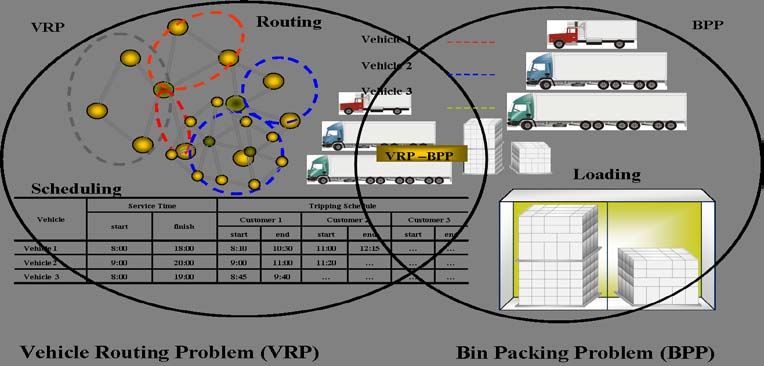
4 Definition of RoSLoP
RoSLoP, immersed in the logistics activity of the company study case, involves a subset of three tasks: routing,
scheduling and loading. The mathematical model of RoSLoP was formulated with two classical problems: routing
and scheduling through VRP and the loading through the Bin Packing Problem (BPP). Fig. 1 shows RoSLoP and its
relation with VRP-BPP.
Computación y Sistemas Vol. 13 No. 4, 2010, pp 398-408
ISSN 1405-5546Construction of an Optimal Solution for a Real-World Routing-Scheduling-Loading Problem 401
Fig. 1. Definition of the Routing-Scheduling-Loading Problem (RoSLoP)
The case of study contains the next elements:
• A set of ORDERS to be satisfied at the facilities of the customers, formed by boxes of products with different
attributes such as weight, high, product type, supported weight, packing type and beverage type.
• A set of n customers with independent service schedules at a facility j [start_servicej, end_servicej] and a finite
capacity of attention of the vehicles.
• A set of depots with independent schedules, which have the possibility to request goods to other depots.
• A fleet of vehicles with heterogeneous capacity Vehiclesd to transport goods, with a service time service_timev and
a time for attention at the facilities of the customers. The attention time tmvj depends on the capacity of the vehicle
and the available people for docking and loading the vehicles.
• A set of roads represented by the edges of the graph. Each road has an assigned cost Cij, each one with a threshold
of allowed weight MAXLoadvj for a determined vehicle v that travels towards a facility j, and a travel time tij from
facility i to j.
The objective of RoSLoP is to get a configuration that allows the satisfaction of the set of ORDERS at the set of
the customer facilities, minimizing the number of vehicles used and the distance traveled. This new formulation
includes a model with 12 variants of VRP: CVRP, VRPTW, VRPMTW, MDVRP, SDVRP, sdVRP, VRPM, HVRP,
CCVRP, DDVRP, rdVRP and OVRP, described in section 2.1.
5 Formulation of RoSLoP
Input sets
C Set of customer facilities or vertex of the associated graph
ORDERS Set orders to be satisfied
D Set of depots to satisfy all the customer demands
Vehiclesd Set of available vehicles in a depot d
K Set of all existent routes in a graph
Kd Set of routes to be covered by a depot d ∈ D
Palletsv Set of containers of a vehicle v. Each container has an associated pair (hpalletij, wpalletij), which
represents the high and weight of a container i when a customer j is visited by a vehicle v.
ITEMSj A set of units of ORDERS for a customer j.
Computación y Sistemas Vol. 13 No. 4, 2010, pp 398-408
ISSN 1405-5546402 Juan Javier González Barbosa, et al.
Parameters
Capacityvj Capacity of a vehicle v to visit a customer j.
service_timev Service time of vehicle v.
tmvj Maneuver time of a vehicle v at facility j, associated to vehicle docking and loading
MAXLoad vj Upper limit for the load to be assigned to vehicle v to visit facility j
MAX Vehicles j Upper limit fot the number of vehicles attended simultaneously at a facility j.
start_servicej The time when a facility j starts its operation
end_servicej The time when a facility j ends its operation
cij Transportation cost to travel from facility i to j
tij Transportation time to travel from facility i to j
Real variables
Loadvj Assigned load in a vehicle v to visit facility j.
arriveik Arrival time of a vehicle to facility i using route k.
leftik Departure time of a vehicle from a facility i using route k.
ϕk Associated cost to travel by route k.
tk Travel cost of a vehicle by route k.
Integer variables
xijk 1 if the edge (i, j) is visited on route k, 0 in otherwise
yvk 1 if vehicle v is assigned to route k, 0 in otherwise
5.1 Preprocessing of the instance of RoSLoP
The preprocessing of an instance is carried out through a linear transformation function, which normalizes the load
objects of the problem. Load objects are defined as n-dimensional objects. They are transformed into a set of real
numbers where each number represents an n-dimensional object. The function of transformation is illustrated in
Fig. 2, in which, an order of a customer j is transformed. This function represents the relationship between the
dimensions of the objects. It consists of two steps: 1) the construction of units of load and 2) the transformation of
these units in a representative set of real numbers.
f : n
→
ITEMS j ∈ n
DiPro algorithm
(boxes of product) (platforms of product)
ITEMS j ∈
ITEMS1 = {0.996, 0.847, 0.498}
Homogeneus Heterogeneus
platforms platforms
1.00*300
=
item1 = 0.996
ITEMS1 1.00 + 300
item height weight 0.85*300
=
item2 = 0.847
1 1.00 300 0.85 + 300
1 2 2 0.85 230
3
0.50*145
3 0.50 145 =
item3 = 0.498
0.50 + 145
Fig 2. Transformation of the orders dataset of the case study
Computación y Sistemas Vol. 13 No. 4, 2010, pp 398-408
ISSN 1405-5546Construction of an Optimal Solution for a Real-World Routing-Scheduling-Loading Problem 403
The construction of load units is done through the DiPro is invoked. As a result, two kinds of units are created:
homogeneous and heterogeneous platforms. Homogeneous platforms are constituted by products of the same type,
while heterogeneous platform are constituted with different types of products with similar characteristics. Both,
Homogeneus and Heterogeneus platforms are defined as a set ITEMSj={ ∀ (wi,hi)}. Then, each pair (wi, hi) is
transformed into a number itemi using the following expression (1). A detailed review of DiPro is presented in [Cruz,
L. et al., 2007b].
hi wi
itemi = i ∈ ITEMS j (1)
hi + wi
The capacity Capacityvj of a vehicle v to visit node j is transformed likewise. Each container that belongs to a
trailer has two attributes: a high hpalletij and weight wpalletij of the assigned load to visit customer j. The width of
the load is determined by a categorization of products, asked the company to group the products. This is necessary
for adjusting the load to the containers. The transformation of the vehicles dimensions is shown in Fig. 3.
Palletsv w h
i=1 375 1.1
i=2 375 1.5
i=3 375 1.5
i=4 375 1.3
Node j
0 1 2 MAX Loadv 2
1
=
wPalleti 2 = 375
0 1000 1500 Palletsv
Node v
1000 0 0
1000
1500 0 0 4 hpalleti 2 wpalleti 2
=
Capacity12 ∑=
h +w
5.379
0 2
i =1 palleti 2 palleti 2
1500
Fig. 3. Transformation of the vehicles dimensions
It is assumed that the weight of the load to be assigned to each container must be uniform. Expression (2) is
used to obtain the capacity of the vehicle. This expression ensures that the dimensions of the load objects and the
vehicles are equivalent.
Palletsv hpalleti j wpalleti j
j ∈ C , v ∈ Vehiclesd
Capacityvj = ∑i =1 hpalleti j + wpalleti j (2)
Load vj = ∑
r∈ITEMS j
itemr ∑
i∈C ∪ D
xijk j ∈ C ∪ D, k ∈ K d (3)
Once defined the input parameters, instance preprocessing is performed. These elements are used to formulate
the integer programming model. The combination of these elements generates the solution to the related rich VRP.
5.2 Mathematical model to solve the rich VRP
The objective of RoSLoP is to minimize the assigned vehicles and the distance traveled, visiting all the customer
facilities and satisfying the demands. Each route k is constituted by a subset of facilities to be visited and a length ϕk .
Computación y Sistemas Vol. 13 No. 4, 2010, pp 398-408
ISSN 1405-5546404 Juan Javier González Barbosa, et al.
Expression (4) is used to get the maximum covering set established by the use of variant HVRP. Expressions (5)-(6)
permit obtaining the length and the travel time on a route k.
max ( ITEMS j )
K d = Vehiclesd Kd ∈ K
min ( Capacityvj )
(4)
ϕk = ∑ ∑
j∈C ∪ D i∈C ∪ D
cij xijk k ∈ K , v ∈ Vehiclesd (5)
=tk ∑ ∑
j∈C ∪ D i∈C ∪ D
tij xijk + ∑ ∑
i∈C ∪ D j∈C ∪ D v∈Veh cles
∑
i d
tmvj xijk yvk k ∈ Kd (6)
The objective function of the problem, defined by expression (7), minimizes the number of assigned vehicles
and the length of all the routes generated. Expressions (8) – (10) are used to generate feasible routes and solve the
related TSP problem. Expression (8) restricts each edge (i, j) on a route k to be traversed only once. Expression (9)
ensures that route k is continuous. Expression (10) is used to optimize the covering set related with the objective
function. These expressions solve variants DDVRP and MDVRP.
min ∑ ∑ ϕk yvk (7)
k∈K d v∈Vehiclesd
(8)
∑
i∈C ∪ D
xijk = 1 k ∈ Kd , j ∈ C ∪ D
∑ ∑ k ∈ Kd , j ∈ C ∪ D
(9)
xijk − x jik =
0
i∈C ∪ D i∈C ∪ D
k ∈ Kd (10)
∑ ∑
i∈C ∪ D j∈C ∪ D
xijk ≥ 1
Expressions (11)-(14), formulated in [5], calculate the time used by a vehicle assigned to route k. Expression
(14) ensures that the use of a vehicle does not exceed the attention time at facility j. These expressions permit solving
the variants VRPTW, VRPMTW and VRPM. The variants CCVRP and SDVRP are solved using the expression
(15), which ensures that two routes k and k’ do not intersect each other at a facility j.
tk yvk ≤ service _ timev k ∈ K d ; v ∈ Vehiclesd (11)
left jk ≥ arrive jk ∑
i∈C ∪ D
tij xijk + ∑
v∈Vehiclesd
tmvj yvk j ∈ C ∪ D, k ∈ K d (12)
arrive jk ∑
i∈C ∪ D
xijk = ∑
i∈C ∪ D
tij xijk j ∈ C ∪ D, k ∈ K d
(13)
start _ service j ≤ arrive jk ≤ end _ service j j ∈ C, k ∈ Kd
(14)
(15)
arrive jk ≤ left jk ≤ arrive jk ' k < k ' , ∀k , ∀k ' ∈ K d
Computación y Sistemas Vol. 13 No. 4, 2010, pp 398-408
ISSN 1405-5546Construction of an Optimal Solution for a Real-World Routing-Scheduling-Loading Problem 405
Expressions (16)-(18), formulated in [1] and combined with the linear transformation function, define the
restrictions for variants CVRP, sdVRP, rdVRP and HVRP. Expression (16) establishes that a vehicle is assigned to a
route k. Expression (17) ensures that vehicle capacities are not exceeded. Equation (18) establishes that all goods
must be delivered and all demands are satisfied. The relaxation of the model that permits the solution of the variant
OVRP consists of the reformulation of expression (9) through expression (19).
∑ yvk ≤ 1 k ∈ Kd
v∈Vehicles
(16)
Load vj ≤ Capacityvj yvk k ∈ K d ; v ∈ Vehiclesd
(17)
ITEMS j − ∑ Load vj =
0 j ∈C ∪ D (18)
j∈C
∑
i∈C ∪ D
xijk − ∑
i∈C ∪ D
x jik ≤ 1 k ∈ Kd , j ∈ C ∪ D (19)
The right side of expression (19) is 0 when a route starts and ends at a depot; otherwise, when the right side has
the value 1 means that route starts at a depot and finishes at a different facility.
6 Experimentation
Real instances were provided by the bottling company. They were solved using the approximate algorithm called
Heuristics-Based System for Assignment of Routes, Schedules and Loads (HBS-ARSL) proposed in [3] and an exact
method. Both were tested on a set of VRP variants that are present in the test data set: VRPTW, VRPMTW, sdVRP,
SDVRP, rdVRP, CCVRP, DDVRP, CVRP y HVRP. The HBS-ARSL algorithm was coded in C# and it was
executed during two minutes to observe the time when it reaches the best solution. The implementation of the exact
method was coded in C# and uses the LINDO API v4.1. A set of 12 test instances were selected from the database of
the company, which contains 312 instances classified by the date of the orders; the database contains also 1257
orders and 356 products in its catalogues. Eight available vehicles were disposed. The results are shown in Table 3.
Table 3. Experimentation with real-world instances, provided by the bottling company
Instance n |K| ORDERS HBS-ARSL Exact method
Distance Vehicles Time Distance Vehicles Time
Traveled Used (secs) Traveled Used (secs)
06/12/2005 4 5 158 1444 4 51.33 1444 3 3.09
09/12/2005 5 5 171 1580 5 23.64 1580 5 3.32
12/12/2005 7 9 250 2500 6 38.52 2500 6 5.03
01/01/2006 6 9 286 2560 7 75.42 2560 6 3.42
03/01/2006 4 4 116 1340 4 63.00 1340 4 2.97
07/02/2006 6 9 288 2660 7 83.71 2660 6 4.53
13/02/2006 5 7 208 1980 5 55.57 1980 5 3.85
06/03/2006 6 7 224 1960 5 32.16 1960 5 3.36
09/03/2006 6 9 269 2570 6 76.18 2570 6 3.85
22/04/2006 8 11 381 3358 7 57.35 3358 7 5.24
14/06/2006 7 8 245 2350 6 90.84 2350 6 4.86
04/07/2006 7 9 270 2640 6 72.49 2640 6 4.53
Average 6 8 238.83 2245.16 5.66 55.27 2245.16 5.33 4.00
Computación y Sistemas Vol. 13 No. 4, 2010, pp 398-408
ISSN 1405-5546406 Juan Javier González Barbosa, et al.
7 Analysis of Results
The exact method obtained the optimal solution for the 12 instances of the test data set; which permits to measure the
performance of the algorithm HBS-ARSL when solving the related rich VRP variant. Table 3 shows that HBS-ARSL
reaches the optimal solution in 100% of the cases considering the distance traveled and in 75% considering the
number of vehicles assigned. These results reveal as consequence, the need of improving the search techniques of
HBS-ARLS to reach 100% of efficiency. The best solutions of HBS-ARLS were obtained in 55.27 seconds on
average, while the exact method reaches the optimal solutions in 4 seconds, permitting a reduction of 92% in
execution time; which reveals the advantages of the transformation function used to reduce the execution time and
the computation of the optimal solution.
8 Conclusions and Future Works
This work presented a mathematical formulation and a linear transformation function, which make possible to obtain
the optimal solution for the rich VRP variant related to RoSLoP. It was demonstrated that, the use of mathematical
artifices can be used to reduce the dimensionality generated by the solution of many VRP variants. This allowed the
obtaining an optimal solution through the formulated integer problem. It could be advantageous when an exact
solution is needed for problems classified as NP-Hard as VRP or BPP. However, this transformation function has the
restrictive condition of the dependence of domain for this application. Therefore, it is proposed the construction of a
transformation function, which is able to reduce the dimension of some specific problems as BPP to a representative
set. This can be used to obtain the optimal solution for other real-world problems.
References
1. Archetti, C., Mansini, R. & Speranza, M.G. (2001). The Vehicle Routing Problem with capacity 2 and 3,
General Distances and Multiple Customer Visits. Operational Research Peripatetic Post-graduate Programme.
1(1),102-112.
2. Bianchi, L. (2000). Notes on Dynamic Vehicle Routing. (IDSIA-05-01). Switzerland: Istituto Dalle Molle di
Studi sull'Intelligenza Artificiale.
3. Cano, I., Litvinchev, I., Palacios R., & Naranjo, G. (2005). Modeling Vehicle Routing in a Star-Case
Transportation Network. Memoria del XIV Congreso Internacional de Computación CIC, IPN. México DF. 373-
377.
4. Cordeau, J.F., Desaulniers, G., Desrosiers, J., Solomon, M.M. & Soumis, F. (1999). The VRP with time
windows. (GERAD G-99-13). Montreal: École des Hautes Études Commerciales de Montréal.
5. Cruz, L., González, J.J., Romero, D., Fraire, H.J., Rangel, N., Herrera, J.A., Arrañaga, B.A. & Delgado,
J.F. (2007a). A Distributed Metaheuristic for Solving a Real-World Scheduling-Routing-Loading Problem.
Symposium on Parallel and Distributed Processing and Applications ISPA 2007. Lecture Notes in Computer
Science, 4742, 68-77.
6. Cruz, L., Nieto-Yáñez, D.M., Rangel-Valdez, N., Herrera, J.A., González, J.J., Castilla, G., & Delgado-
Orta, J.F. (2007). DiPro: An Algorithm for the Packing in Product Transportation Problems with Multiple
Loading and Routing Variants. Mexican International Conference on Artificial Inteligence MICAI 2007. Lecture
Notes in Computer Science, 4827, 1078-1088.
7. Cruz, L., Delgado-Orta, J.F., González, J.J., Torres, J., Fraire, H.J., & Arrañaga, B.A. (2008). An Ant
Colony System to solve Routing Problems applied to the delivery of bottled products. International Symposium
ISMIS 2008. Lecture Notes in Computer Science, 4994, 329-338.
8. The VRP Web. (2005). Retrieved from http://neo.lcc.uma.es/radi-aeb/WebVRP.
9. Fleischmann, B. (1990). The Vehicle routing problem with multiple use of vehicles. Hamburg: Universitt
Hamburg.
Computación y Sistemas Vol. 13 No. 4, 2010, pp 398-408
ISSN 1405-5546Construction of an Optimal Solution for a Real-World Routing-Scheduling-Loading Problem 407
10. Goel, A. & Gruhn, V. (2005). Solving a Dynamic Real-Life Vehicle Routing Problem. Operations Research
Proceedings, 1(1), 367-372.
11. Flatberg, T., Hasle, G., Kloster, O., Nilssen, E.J., & Riise, A. (2007). Dynamic and Stochastic Vehicle
Routing in Practice. Operations Research/Computer Science Interfaces Series, 38(1), 45-68.
12. Herrera, J. (2006). Development of a methodology based on heuristics for the integral solution of routing,
scheduling and loading problems on distribution and delivery processes of products. MSc Thesis. Instituto
Tecnológico de Ciudad Madero, Tamaulipas, México.
13. Jacobs, B. & Goetshalckx, M. (1993). The Vehicle Routing Problem with Backhauls: Properties and Solution
Algorithms. (MHRC-TR-88-13). Georgia: Georgia Institute of Technology .
14. Mingozzi, A. (2005). The Multi-depot Periodic Vehicle Routing Problem. Symposium Abtraction,
Reformulation and Approximation SARA 2005. Lecture Notes in Computer Science, 3607, 347-350.
15. Pisinger, D. & Ropke, S. (2005). A General Heuristic for Vehicle Routing Problems. Computers & Operations
Research, 34(8), 2403-2435.
16. Rangel, N. (2005). Analysis of the routing, scheduling and loading problems in a Products Distributor. MSc
Thesis. Instituto Tecnológico de Ciudad Madero, Madero, Tamaulipas,México.
17. Shaw, P. (1998). Using Constraint Programming and Local Search Methods to Solve Vehicle Routing
Problems. Principles and Practice of Constraint Programming – CP98. Lecture Notes in Computer Science.
1520, 417-431.
18. Taillard, E. (1996). A Heuristic Column Generation Method For the Heterogeneous Fleet VRP. (CRI-96-03).
Switzerland: Istituto Dalle Moli di Studi sull Inteligenza Artificiale.
19. Thangiah, S. (2003). A Site Dependent Vehicle Routing Problem with Complex Road Constraints. (SRT84-
2003) Slippery Rock University, PA.
20. Toth, P. & Vigo, D. (2001). The vehicle routing problem. SIAM, Monographs on Discrete Mathematics and
Applications. Philadelphia: Society for Industrial and Applied Mathematics.
Juan Javier González Barbosa. He received the Ph.D. in computer science from the Centro Nacional de
Investigación y Desarrollo Tecnológico, Cuernavaca, México in 2006. His scientific interests include metaheuristic
optimization and machine learning.
José Francisco Delgado Orta. He received the MSc degree in computer sciences from the Instituto Tecnológico de
Ciudad Madero, Ciudad Madero Tamaulipas, México in 2007. He is a systems consultant with professional activity
in Mexico.
Computación y Sistemas Vol. 13 No. 4, 2010, pp 398-408
ISSN 1405-5546408 Juan Javier González Barbosa, et al. Héctor Joaquín Fraire Huacuja. He received the Ph.D. in computer science from the Centro Nacional de Investigación y Desarrollo Tecnológico, Cuernavaca, México in 2005. His scientific interests include metaheuristic optimization and machine learning. José Antonio Martínez Flores. He received the Ph.D. in computer science from the Centro Nacional de Investigación y Desarrollo Tecnológico, Cuernavaca, México in 2006. His scientific interests include distributed database design and natural language processing. María Lucila Morales Rodríguez is professor at the Instituto Tecnológico de Cd. Madero, Mexico. She received a Ph.D.degree in Informatics from Université Paul Sabatier, France in 2007. She has conducted research in virtual characters and emotional interfaces. Computación y Sistemas Vol. 13 No. 4, 2010, pp 398-408 ISSN 1405-5546
You can also read