Introduction to Terrestrial Laser Scanning (TLS) - UT Dallas
←
→
Page content transcription
If your browser does not render page correctly, please read the page content below
Introduction to Terrestrial Laser
         Scanning (TLS)
• Similar to Sonar and Radar but uses Light (Light
  Detection and Ranging)
• Initial of LiDAR use began in the 1960’s in studies of
  atmospheric composition, surveying, law enforcement,
  etc.
• Transmits a pulse of light and records the returned pulse
  of light – records time, divides by two, and multiplies by
  the speed of light for distance
• Able to record thousands of points a second recording
  target position (X,Y,Z), intensity, and color (RBG)
• Capable of relative positioning at mm to cm accuracy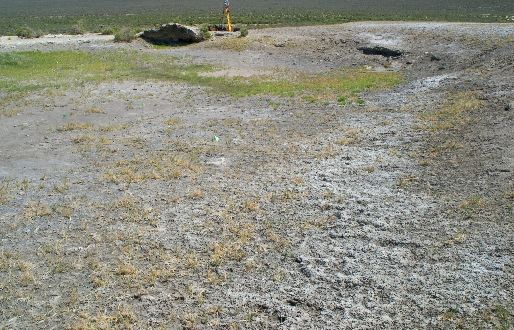
LASER SCANNERS
• Beam deflection mechanism provides elevation and azimuth
  of the transmitted pulse

• Return-beam detection device records return time and
  provides range calculation from two-way travel time

• Energy of the return pulse (intensity) and the color (RBG) is
  recorded

• Full waveform now recorded on some TLS instruments
Time-of-Flight Measurement

     Transmitter

      Receiver

             Range = travel time x speed of light/2
             Record (azimuth, zenith, range, intensity)

Greaves, SPAR 2004.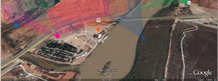
BENEFITS OF LASER SCANNERS
• Imaging system provides an unprecedented density of
  geospatial information through a dense set of three-
  dimensional vectors to target points relative to the
  scanner location (point cloud)

• Scanner controlled by laptop computer that is also used
  for data acquisition and initial processing

• Combination with GPS allows fully geospatially
  referenced data set and opens potential for direct
  measurement of change (time series measurements)
3D POINT CLOUD
• Cartesian transformation of the laser pulse data (trans-
  formation of the range and reflectance images as well as
  the calculated XYZ coordinates) in scanner centered
  reference frame

• 3D point cloud of discrete locations derived from
  superimposing range and reflectance image for each laser
  pulse

• 3D point clouds are the basis for subsequent analysis and
  used to create CAD or GIS models
REFLECTANCE IMAGE
• Looks like a black and white photograph of scan
  coverage

• Individual measured points are defined as
  reflectance values
   – highly reflecting (light) points are displayed in a
     light grey pixel
   – highly absorbing
      (dark) points are displayed as a dark grey pixel
   – lack of a return is depicted as a black pixel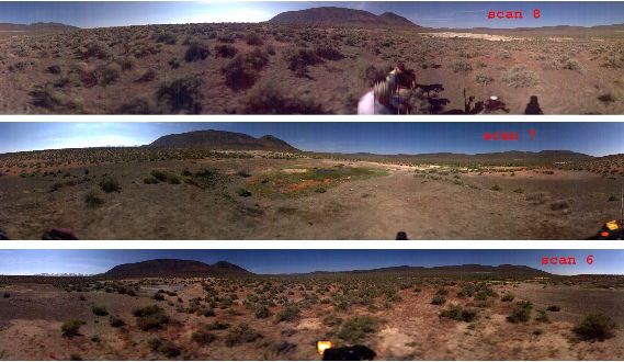
Field Equipment

                Laptop

                                   Terrestrial
                                     Laser
Controls to                         Scanner
align all the                      (LPM 800)
 scanning
    data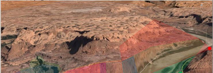
Field Equipment

               Camera                     Tripod
   Topcon                  RTK GPS
Totalstation
  Imagine
  System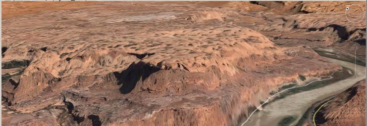
Integrating geometry with texture by position
                       control

                                       Camera
                                 GPS                          Imaging Total Station

                                         Nikon D200

                                                               OR
TOPCON HIPER LITE+ - RTK GPS SYSTEM

                                                                          TOPCON IS
                     Total Station
                                       TOPCON Total Station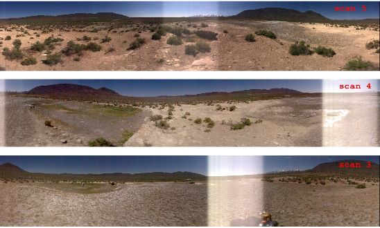
Examples of controls
Scanner Parameters
•   Beam Divergence
•   Angular Step
•   Range Distance
•   Field of View
•   Points Per Second
•   Size and Weight
Scanner Parameters
• Beam Divergence
  Df = (Divergence * d) + Di
Scanner Parameters
Scanner Parameters
• Angular Step
  Spacing = d(m)*TAN(step)
Scanner Parameters
Scanner Parameters
• Range Distance
  Target Reflectance can change single scan range by hundreds of meters
  Laser and CCD characteristics impact maximum and minimum range
  distances from 2000 (6000) meters

• Field of View
  Rotational Base allows 360 degree rotation (azimuth)
  Rotating mirror and gear drive allows ~90 degree vertical coverage

• Points Per Second
  Scan Time

• Size and Weight
  Field Logistics
Beam Stepping Distance
• Beam stepping angle is specified in either degrees/minutes/seconds, in
  decimal degrees or in gons. There are 400 gons in a circle, just as there
  are 360 degrees in a circle.

• Unfortunately, the specs units are not radians (2π radians in a circle). If
  they were radians, a very rapid approximation of the stepping distance in
  meters can be made mentally. For small angles,
       Stepping Distance = (angle in radians) * distance
       e.g. Stepping Angle = 0.00005 radians (.05 mRadians)
            Stepping Distance (@800m) = 0.00005* 800 = 4 cm

         1 gon = 0.9 deg             1 deg = 1.111 gon
       1 deg = 0.01745 radians

• Minimum specs for stepping tend to be 0.0012 => 0.004 deg
        0.002 deg = 0.035 mRadians = 3.5 cm at 1000 meters
Beam Divergence
• Beam Divergence
– Optech Ilris 0.00974 deg (0.17 mRadian)
– Riegl LMS 620i 0.004 deg (0.07 mRadian)
– Riegl LPM 321 0.046 deg (0.8 mRadian)
• Beam diameter at exit ranges from a few millimeters to centimeters
• Spot diameter at distance
diameter = beam at exit + divergence (radians) * distance
Riegl 620 = 2 mm + (0.00007 radians * 500 m) = 3.7 cm
Riegl LPM = 1 cm + (0.0008 radians * 500 m) = 41 cmLaser Return Signal
BeamDiameterAtOutcrop = divergence * distance Beam size at laser = 1 cm2
Beam divergence = 0.8 mrad
= 0.0008 * 50000 cm = 40 cm
Beam intensity at laser = 1 cm-2
2
BeamAreaAtOutcrop = (BeamDiamter / 2) * π Distance to outcrop = 500 m
Reflectivity = 33%
2
= (40 / 2) * π = 1257 cm 2
IntensityAtOutcrop = InitialBeamIntensity / BeamAreaAtOutcrop
= 1 / 1257 = 0.0008 cm -2
Re turnAtOutcrop = ObjectArea * IntensityAtOutcrop * Reflectivity
= 100 * 0.0008 * 0.33 = 0.26
(
ReturnIntensityAtLaser = ReturnAtOutcrop/ 2 * π * distance 2 )
2 −11 2
= 0.26 /(2 * π * 50000 ) = 1.66 cm
= 0.0000000000166
The return signal at the laser is substantially lower than the signal that is
emitted by the laser.
The example above assumes that the laser beam is 1 cm2 when it leaves the
laser and that the window to the receiver has an aperture area of 1 cm2 and
that the feature being imaged is 100 cm2.Diffuse reflection for reflectorless laser
rangefinders
Laser beam
with 3 milliradian div. Target
Laser range- receiver aperture
finder
diffuse reflection
Not to scale904 nm diffuse fractional reflections
of common material
Other lasers have different responses when operating at different wavelengths
Material Description DR.
Winter Snow and Ice 0.85
Vegetation (The Average Value of Many Types) 0.50
Soil 0.05 - 0.35
Silt 0.20 - 0.40
Sand 0.10 - 0.35
Gypsum 0.55 - 0.70
Clay 0.40 - 0.50
Dirt 0.30
Shale, Coral 0.45
Concrete, Asphalt 0.10
Coal Tar Pitch 0.05
Plywood, Unpainted 0.50
Brick, Red 0.25
Bark 0.20 - 0.25Range Measurement versus Intensity
CD Reflectors Mounted on a Wall
Note angle of points from wall pointing toward scannerRange Error versus Intensity LIDAR emits a short pulse of light and measures the time for the return signal to reach the detector. Light travels at about 0.33 m / ns in air. Distance = ½ * time of flight * velocity of light. Enough returned energy must be received at the LIDAR detector to trigger the timing circuitry. If the signal is very strong, the detector threshold will be reached faster than if the signal is very weak. LIDAR detectors must compensate for this effect in order to provide accurate measurement of distance.
LASER SCANNER ACCURACY
• Boehler, Vincent and Marbs, 2003.
• Tested scanners for accuracy
• Application was for cultural heritage
  applications (we will revisit for natural
  surfaces)
• Manufacturer specifications not good
  representation for real-world applications
LASER SCANNER ACCURACY
• Angular accuracy
  – Angles from combination of deflection of rotating
    mirrors and rotation about a mechanical axis
  – Provides azimuthal position
• Range accuracy
  – Time of flight or phase comparison between
    outgoing and returning signal provides range
  – Noise-fuzz of points on a flat surface
LASER SCANNER ACCURACY
• Resolution
– Ability to detect an object in point cloud
– Two specs contribute
• Smallest increment of angle between successive points
(can manually set)
• Size of laser spot (beam dispersion)
• Edge effects
– When a spot hits the edge of a target and receives
2 positions and/or 2 reflectivity values (material)LASER SCANNER ACCURACY
• Surface reflectivity
– Distance, atmospheric, incidence angle
– Albedo (ability to reflect)
• White strong, black weak
• Depends on spectra of the laser (green, red, near IR)
• Inclined surfaces of high reflectance (i.e., water ) can
create travel time anomalies (mutlipathing)
– Typically contribute accuracy-range errors larger
than manufacture specificationsEnvironmental Conditions
• Temperature (important to operate within
specification range)
• Atmosphere
– changes propagation speed slightly
– dust, mist, raindrops, fog - a major problem
• Interfering radiation
– Sunlight strong relative to signal
• Influence or prevent (don’t shoot into sun)Survey Control • Surface referencing (using recognizable physiographic features) • Targets (reflectors and/or prisms) • Geo-referencing (Total Station and GPS positioning) • Multiple scan registration requires tight spatial control
Calibration
• Repeatability
  – Need to document multiple measurements of
    known geometry
  – Compare with allowable variance
• Quality Control
  – Multiple measurements of known geometry with
    multiple scanner positions
Resolution • Measurement accuracy is governed by instrument resolution • Resolution is the smallest distance that can be measured without ambiguity • For laser scanning, this is the spacing of the point cloud array • Varies linearly with distance from the scanner
Resolution

   Range
Measurement Accuracy
• The ability to generate physical dimensions
  and location of an object
  – Specified with a tolerance, e.g. +/- 6 mm
    (and a confidence interval)
  – Not a laser scanner specification but a work
    product specification
Resolution and Measurement Accuracy • Absolute measurement accuracy can’t be better than 2x instrument resolution
Resolution and Measurement Accuracy

• Absolute measurement accuracy can’t be
  better than 2x instrument resolution
Resolution and Measurement Accuracy

• Modeling may help, caution required
Resolution and Measurement Accuracy

• Overlapping dot problem (edge effect)
Resolution test
Measuring noise in range direction. Riegl Z420 is
             comparable to Z360
Action Sequence in the Field
• First, establish the scan locations and ensure that they completely cover the target
area.
• Second, establish the location for the controls
• Third, review naming and number conventions to be used
• Make sure that the site name in the software and the folder and site abbreviation
in the camera set is correctly set (can be done night before)
• Set up controls and locate them with GPS (time series measurement reduce errors)
• Set up first scan site and decide on camera sites (if applicable)
• Scan controls before scanning the outcrop
• The photo team with the Topcon IS needs to be working in parallel with the scan
team. One can get ahead of the other, but the jobs need to proceed in parallel. It
takes a lot of time.
• Review the progress with one another
• Double check the work
• Save all work to an archive file that is not used as a work file
• Review the data in the field if possible
• Start model construction as soon as possible in order to correct errors or fill in
unintentional holes in the dataLiDAR Site Selection
(multiple locations, selection of point density versus time)
• It is necessary to scan an outcrop from at least two oblique
directions to minimize occluded parts of the outcrop. Three
scans are good (left/center/right), and additional reverse
directions are optimal.
• Point density is inversely dependent upon distance to the
outcrop. If the distance has a wide range of values, the time
to scan the outcrop can be optimized by selecting a finer
angular resolution for the more distant parts of the outcrop
compared to the closer parts of the outcrop.
– Scan time is inversely dependent upon the square of the scan angluar
resolution. Increasing the scan step angle by 2X reduces the scan time
by 4X.
– Partition the outcrop scans to maintain a nearly uniform linear
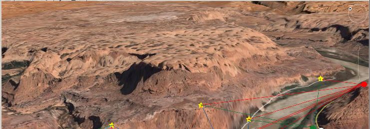
stepping distance at the outcrop surface.Scan Positions
overhang
Choose scan positions to minimize occluded (shadowed or hidden)
geometries. Scanner blue will not image beneath the overhang or
the right side of the overhang. Scanner red will image underneath the
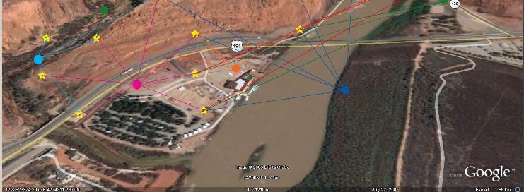
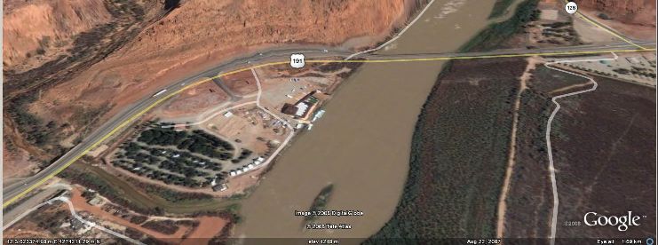
overhang and will image the right side of the overhang.Moab Utah-Google Earth Screen Capture
Multiple Scan Positions

        Moab Utah
Scan Partition as a Function of Range
Scan Partition as a Function of Angle of Incidence
Scan Partitioning Avoids Unnecessary Scan Time
Scan Partitioning

Scan of the “Pyramid” at Slaughter Canyon, Carlsbad Caverns National
Monument, New Mexico
          Scanner was on a 200m high hill.
          Scan ranges were 50m to 800m
Scan Partitioning Scanning of the total outcrop at the scan step angle needed for the longest scan would have dramatically increased the scan time. Scanning the outcrop in a single scan which covered the entire outcrop would Result in a large amount of empty data.
Placement and Survey of the Controls
• Use of scanned control reflectors improves the accuracy of the model and
  allows straight forward alignment of the individual scans
• Alignment of two scans requires an absolute minimum of three control
  points. It is best to have five or more available to accommodate errors.
• If multiple scan sites are used, it is not necessary to have all control
  reflectors visible from all of the scan sites. However, it is necessary that
  each scan site be able to see at least three reflectors that have been
  correlated with other scan sites
• The control reflectors should cover a wide area (preferably surrounding
  the image area), do not place reflectors in a linear fashion or group them
  in a tightly.
• The spacing of the reflectors optimally approximates or exceeds the
  distances in the scan region. However, this may not be practical.
• It is not necessary to have reflectors on the outcrop and/or within the
  image area, although it is desirable to do so if practical and is aesthetically
  acceptable (for photorealistic analysis).
Placement and Survey of the Controls
Scan Reflectors before Scanning Outcrop
• It is prudent to scan the reflectors before scanning the
  outcrop.
   – If you do not have the controls with the scan data, you may not be
     able to use the scans
   – If something happens to disorient the scanner or there is a power or
     software crash during the subsequent scans, the work up to that point
     can still be used
   – For double protection, rescan at least some of the reflectors after
     completing the outcrop scan. If the scanner has lost alignment, the
     final reflector scan will identify the problem.
• When using the LPM with the telescopic sight, the scan
  window must be larger than expected. There is parallax
  between the scanner and the telescope. This is a much larger
  problem at close range than at long range.
Collecting Field Data
GPS Control
Scan Pos 1
GPS
Photo ControlCollecting Field Data
Scan Pos 1
GPSCollecting Field Data
Scan Pos 1
GPSCollecting Field Data
GPS
Scan Pos 2Collecting Field Data
GPS
Scan Pos 2Collecting Field Data
GPS
Scan Pos 2Collecting Field Data
Photos
Photos
PhotosGeospatial Referencing: GPS
Summary of the approximate accuracy of GPS positioning versus methods. (Modified from
Featherstone, 1995)High-Resolution Geospatial Referencing: GPS
and Total Station
• Accurate measurement of reference network
baselines with Total Station (mm)
• Time series measurement of individual reference
reflectors/prisms with continuous GPS (cm)
• Simultaneous GPS solution of all reference sites and
network adjustment using TS baselines to provide
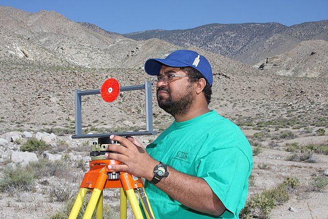
sub-cm resultsMickey Hot Springs, SE Oregon
ZOOM OF DOQ
Problem: map a flat terrain and generate a cm level terrain map not feasible with airborne methods
DETAILED
AREA
470MZOOM of DOQ
Riegl Z360 mapping fairly flat surface
Actual examples of scans at MHS with RGB
channel so points are colored (not external
                 camera)
Scans 2, 3 and 4 are of detailed areas
Scans in southern area
Rotation of initial scan.
   Note vegetation
Another perspective. Note shadows with
              no points.
Perpendicular perspective
Example of merged scans
   (reflectance image)
Color Version
Merged surface fit
You can also read