Cross-Border Spillovers from Fiscal Stimulus
←
→
Page content transcription
If your browser does not render page correctly, please read the page content below
Cross-Border Spillovers from Fiscal Stimulus∗

   Giancarlo Corsetti,a André Meier,b and Gernot J. Müllerc
   a
       European University Insititute, University of Rome III and CEPR
                       b
                         International Monetary Fund
                      c
                        University of Bonn and CEPR

            The global recession of 2008–09 has revived interest in the
        international repercussions of domestic policy choices. This
        paper focuses on the case of fiscal stimulus, investigating cross-
        border spillovers from an increase in exhaustive government
        spending on the basis of a two-country business-cycle model.
        Our model allows spillovers to be affected by a range of fea-
        tures, including trade elasticities, the size and openness of
        economies, and financial imperfections. Beyond these well-
        known determinants, however, we highlight the central impor-
        tance of policy frameworks, notably the medium-term debt
        consolidation regime. We consider the plausible case in which
        a temporary debt-financed increase in government spending
        gives rise to higher future taxes along with some reduction
        in spending over time. The anticipated spending reversal not
        only strengthens the domestic stimulus effect but also enhances
        positive cross-border spillovers through its impact on global
        long-term interest rates. Thus, our findings lend support to
        the notion that coordinated short-term stimulus policies are
        most effective when coupled with credible medium-term con-
        solidation plans featuring at least some spending restraint.
        JEL Codes: E62, F42.

    ∗
      We thank our discussant Volker Wieland and the participants in the con-
ference on Monetary Policy Challenges in a Global Economy organized by the
International Journal of Central Banking and hosted by the Banque de France
(September 24–25, 2009) for excellent comments. Ida Maria Hjortso provided
superb research assistance. Corsetti and Müller gratefully acknowledge generous
financial support from the Fondation Banque de France and the Pierre Werner
Chair Programme on Monetary Union. The views expressed in this paper are
those of the authors and do not necessarily represent those of the IMF or IMF pol-
icy. Please address correspondence to giancarlo.corsetti@eui.eu, ameier@imf.org,
or gernot.mueller@uni-bonn.de.

                                        5
6           International Journal of Central Banking                 March 2010

1.   Introduction

The debate on the appropriate government response to the dramatic
global recession of 2008–09 has revived classical controversies about
fiscal policy. Arguments rage over the size of fiscal multipliers (e.g.,
Cogan et al. 2009, Romer and Bernstein 2009, or Uhlig 2009), as well
as the magnitude of international spillovers from fiscal stimulus at
the national level. According to the received wisdom, domestic fis-
cal stimulus benefits foreign output and employment via increased
demand for imports as the home country’s real exchange rate appre-
ciates. A coordinated fiscal expansion, the traditional argument goes,
can internalize this effect, balancing demand leakages and prevent-
ing unwelcome exchange rate fluctuations. However, there are also
forces counteracting positive spillovers across countries. In particu-
lar, domestic fiscal stimulus (in large economies) may raise global
interest rates and thus dampen foreign activity; this effect will be
even more pronounced if fiscal expansions are debt-financed and
public debt is already high.
    Whatever their net effect, potential spillovers from fiscal expan-
sions (as well as the ensuing “exit strategies”) are high on the agenda
of international policy discussions.1 As a contribution to the ongoing
debate on fiscal policy, this paper analyzes systematically the inter-
national spillover effects of short-term fiscal stimulus. Our modeling
framework allows spillovers to be affected by a range of relevant
factors, such as trade elasticities, openness, or financial imperfec-
tions, but our particular interest is on the regime of medium-run
debt consolidation. Specifically, our analysis departs from the sim-
plistic assumption that higher government outlays today will be fully
offset by higher (future) taxation alone. Instead we allow for a real-
istic response to debt of both taxation and government spending,
implying that at least some of the current fiscal stimulus is paid for
through future expenditure cuts.2

   1
     The IMF, for example, has repeatedly called on its members to coordinate
their policies in response to the crisis, regarding not only the design of effective
short-run measures but also the identification of fiscal consolidation strategies;
see Spilimbergo et al. (2008).
   2
     In previous work (Corsetti, Meier, and Müller 2009a), we have documented
the empirical relevance of such a feedback channel for the United States and
shown how it enhances the short-term expansionary effects of government spend-
ing on domestic activity. This paper extends our analysis to the question of
cross-border spillovers from fiscal stimulus.
Vol. 6 No. 1         Cross-Border Spillovers from Fiscal Stimulus            7

    We carry out our analysis using a two-country business-cycle
model, drawing on earlier work by Backus, Kehoe, and Kydland
(1994) and Chari, Kehoe, and McGrattan (2002), among others.
This stylized model allows us to provide a sharp characterization
of our main results. An exogenous increase in government spend-
ing financed entirely by (current or future) taxes—the experiment
typically analyzed in the literature—causes output to expand and
private consumption to fall.3 The home currency appreciates in real
terms and induces expenditure switching toward foreign goods. Yet
this positive effect on demand for foreign goods is counteracted by a
contraction of global private absorption due to rising interest rates
(unless the domestic economy is very small). Overall, the effect on
foreign activity is quite contained or even negative, depending on
the exact parameterization of the model.
    The model predictions change profoundly under an alternative
medium-term fiscal regime where not only taxes but also government
outlays adjust systematically to consolidate public debt over time.
In this case, the initial debt-financed increase in exhaustive govern-
ment spending triggers a subsequent spending reversal, defined as
a reduction of government spending below trend that partially off-
sets the detrimental effect of the initial fiscal expansion on public
finances. Such dynamics can arise, even in the absence of credible
commitment mechanisms, from de facto constraints on governments’
capacity to raise taxes beyond voters’ tolerance level.4 Spending
reversals, in turn, generate expectations of a fall in future real short-
term interest rates, which immediately affect today’s long-term real
rates, both domestically and, to the extent that the home economy
is large relative to the rest of the world, globally. Provided that
domestic and foreign monetary policy exhibit a measured response
to inflation and the output gap, long-term rates actually fall on
impact, inducing a considerable increase in domestic and foreign
output. Remarkably, the home real exchange rate depreciates in this

   3
     As customary, we consider only the case of lump-sum taxation. Anticipation
of higher distortionary taxes can lead to a wide range of responses, especially
regarding individual components of aggregate demand.
   4
     The Californian electorate’s resistance to higher taxes, expressed in the
famous Proposition 13, is but one particularly striking example of such con-
straints.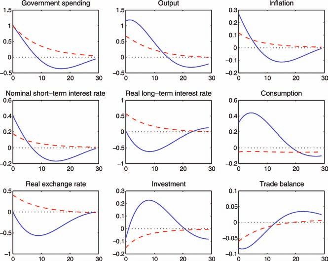
8           International Journal of Central Banking                March 2010

case—in sharp contrast to the prediction under a purely tax-based
debt-consolidation strategy, but matching the time-series evidence.5
    Our analysis thus highlights the importance of debt-consolidation
regimes for the fiscal transmission mechanism, at both the national
and the international level. At the core of the transmission mecha-
nism lies the impact of spending reversals on global financial mar-
kets: the anticipated fall of spending below trend prevents, or at least
contains, increases in global long-term real interest rates and thus
allows the temporary fiscal expansion to stimulate private absorp-
tion worldwide. From the viewpoint of supporting global demand
during the current global recession, our findings confirm the promise
of combining short-term stimulus with clear and credible communi-
cation on (at least partial) expenditure-side consolidation over the
medium term.
    As an important corollary of our results, we find no more than
a limited role for expenditure switching effects from exchange rate
movements. This qualifies commonly cited concerns about unfair
gains in competitiveness accruing to countries that do not imple-
ment a fiscal expansion. According to the conventional wisdom, an
appreciation of the currency of the stimulus country would enable
such “fiscal free-riders” to gain a larger share of foreign markets.
In our analysis, by contrast, real appreciation is neither a necessary
result of domestic fiscal stimulus nor even a primary determinant of
spillovers on foreign economic activity. In fact, our analysis shows
domestic stimulus to trigger a real depreciation under spending
reversals; yet such a policy simultaneously induces sizable positive
output spillovers abroad.
    To the extent that government spending is actually used to sta-
bilize public debt, our findings square well with results from empir-
ical analyses of spillovers. Canzoneri, Cumby, and Diba (2003), for
instance, identify fiscal shocks within a VAR framework and find
a delayed but sizable increase in French, Italian, and British out-
put in response to U.S. fiscal expansions. Beetsma, Giuliodori, and
Klaasen (2006) combine a VAR model with an estimated trade

   5
     A host of time-series analyses have documented real depreciation in response
to fiscal expansion for the United States, the United Kingdom, and Canada; see
Kim and Roubini (2008), Monacelli and Perotti (2006), and Ravn, Schmitt-Grohé,
and Uribe (2007).
Vol. 6 No. 1 Cross-Border Spillovers from Fiscal Stimulus 9
equation for European countries and find sizable output spillovers
from shocks to German and French government spending. Cwik and
Wieland (2009), in turn, use a multicountry model to explore the
likely consequences of the fiscal packages legislated in Europe in late
2008/early 2009. They find that output spillovers from fiscal expan-
sions in Germany to France and Italy are small or even negative.
Although seemingly at odds with our own results, this theoretical
prediction is actually consistent with our analysis, insofar as Cwik
and Wieland consider a time path for fiscal policy that does not
feature any spending reversals.6
The remainder of this paper is structured as follows. Section 2
outlines the model structure. Section 3 discusses the parameteri-
zation of the model and provides results from various simulations.
Section 4 concludes.
2. Model Structure
In this section we outline a two-good, two-country business-cycle
model, similar to Chari, Kehoe, and McGrattan (2002). We assume,
however, that prices and wages are sticky and adjusted à la Calvo.
We also allow for the possibility that a fraction of households is
excluded from financial markets, as in Erceg, Guerrieri, and Gust
(2006) and Bilbiie, Meier, and Müller (2008), among others—a way
to capture financial frictions which may motivate the resort to fis-
cal policy as a stabilization tool. In addition to these “Keynesian”
features, we assume that financial markets are incomplete at the
international level, with trading restricted to non-contingent bonds.
We posit an endogenous discount factor to ensure stationarity of
equilibria. Lastly, we allow for differences in country size and for the
possibility that the composition of final goods depends on their use
for either private or public consumption.7
6
These authors also point out the importance of the exchange rate regime
for the strength of fiscal spillovers; see also Wieland (1996). We explore the
interaction of exchange rate and debt-stabilization regimes in shaping the fiscal
transmission mechanism in a companion paper; see Corsetti, Meier, and Müller
(2009b).
7
Corsetti and Müller (2006) provide evidence for the empirical relevance of
such a distinction.10 International Journal of Central Banking March 2010
The world economy consists of two countries. The countries
may differ in size but are otherwise symmetric, so that in steady
state, per capita quantities are identical across countries and trade
is balanced. In what follows we denote the population of country
i ∈ {1, 2} by Ni and measure the size of country 1 on the unit inter-
val: ς = N1 /(N1 + N2 ). We also refer to country 1 as the domestic
economy or as “Home” and to country 2 as “Foreign.” The following
subsections detail, in turn, the economic choices faced by agents in
the two economies, the conduct of monetary and fiscal policies, and
the relevant market-clearing conditions.
2.1 Final-Good Firms
Final goods—used for either private consumption, investment, or
government consumption—are bundles of intermediate goods. The
bundles are assembled by final-good firms, which operate under per-
fect competition and minimize the cost of combining intermediate
goods. These goods, in turn, are produced by a continuum of monop-
olistically competitive firms in both countries. We use j ∈ [0, 1] to
index these firms (as well as their products and prices).
Let Fit , with F ∈ {C, X, G}, denote, respectively, the final goods
used for household consumption, investment, and government con-
sumption in country i at time t. Further, let Ait (j) and Bit (j) denote
the amount of intermediate good j originally produced in country 1
and 2, respectively, that is subsequently used in country i to assem-
ble some final good F . The specific final-good baskets are defined as
follows:
⎧⎡ ⎤σ−1
σ
⎪
⎪
σ−1
⎪
σ
⎪ 1
1 −1 −1
⎪
⎪ ⎢ (ω1F ) σ A1t (j) dj ⎥
⎪
⎪ ⎢ 0 ⎥
⎪
⎪ ⎢ σ−1 ⎥ , for i = 1
⎪
⎪ ⎣ σ ⎦
⎪
⎨ + (1 − ω1F ) σ
1 1 −1
B1t (j) dj
−1
0
Fit = ⎡ ⎤σ−1
σ
⎪
⎪
σ−1
⎪
σ
⎪
⎪ ⎢
1
(ω2F ) σ
1 −1
B2t (j) dj
−1
⎥
⎪
⎪ ⎢ 0 ⎥
⎪
⎪⎢ σ−1 ⎥ , for i = 2,
⎪
⎪ ⎣ σ ⎦
⎪
⎪ 1
⎩ + (1 − ω ) σ
1 −1 −1
2F 0
A (j) dj
2t
(1)Vol. 6 No. 1 Cross-Border Spillovers from Fiscal Stimulus 11
where σ measures the elasticity of substitution between foreign and
domestic intermediate goods and measures the elasticity of substi-
tution between intermediate goods produced within the same coun-
try. The parameter ωiF measures the average weight of domestically
produced intermediate goods in final good Fit .
Let PitA (j) denote the price in country i of a generic intermedi-
ate good produced in country 1 and let PitB (j) denote the price in
country i of a generic good produced in country 2. Then, letting Et
denote the nominal exchange rate and assuming that the law of one
price holds, we have
B B A A
P1t (j) = P2t (j)/Et ; P1t (j) = P2t (j)/Et . (2)
The price indices for final-good baskets are given by
A 1−σ B 1−σ 1−σ
1
F ω1F P1t + (1 − ω1F ) P1t , for i = 1
Pit = A 1−σ B 1−σ 1−σ
1 (3)
(1 − ω2F ) P2t + ω2F P2t , for i = 2,
where
1
1
1−
1
1
1−
PitA = PitA (j)1− dj and PitB = PitB (j)1− dj (4)
0 0
denote the producer price index (PPI) in Home and Foreign, respec-
tively. As final-good firms minimize expenditures in assembling
intermediate goods, aggregate domestic and foreign demand for
domestically produced goods is given by
⎧ A −σ
⎨ P1t
F ∈{C,X,G} ω1F P1t F F1t , for i = 1
Ait = A −σ (5)
⎩ P2t
F ∈{C,X,G} (1 − ω2F ) P F F2t , for i = 2.
2t
Analogously, aggregate domestic and foreign demand for intermedi-
ate goods produced abroad is given by
⎧ B −σ
⎨ (1 − ω )
P1t
F1t , for i = 1
F ∈{C,X,G} 1F F
P1t
Bit = B −σ (6)
⎩ P2t
F ∈{C,X,G} ω2F P F F2t , for i = 2.
2t12 International Journal of Central Banking March 2010
Note that A2t and B1t correspond to domestic exports and imports
in terms of per capita values of country 2 and country 1, respec-
tively. Global demand for a generic good j produced in country i,
measured in per capita terms, is then given by
⎧ A −
⎨ P1tA(j) A1t + NN1 A2t , for i = 1
2
P
Yit (j) = B1t −
D
(7)
⎩ P2t (j) N1
B + B , for i = 2.
PB N2 1t
2t
2t
2.2 Intermediate-Good Firms
In each country, there is a continuum of intermediate-good firms. A
generic firm j ∈ [0, 1] in country i engages in monopolistic compe-
tition, facing the demand function (7). The production function is
assumed to be of the Cobb-Douglas type:
Yit (j) = Kit (j)θ H̃it (j)1−θ , (8)
where Kit (j) and H̃it (j) denote, respectively, the capital and labor
services employed by firm j on a period-by-period basis. Both factors
may be adjusted freely in each period. Letting Wit denote the price
of labor services and Rit the rental rate of capital, cost minimization
implies H̃it (j)/Kit (j) = (1 − θ)Rit /(θWit ), such that marginal costs
are independent of the level of production and identical across firms:
Wit1−θ Rit
θ
M Cit = . (9)
θ (1 − θ)
θ 1−θ
We assume that price setting is constrained exogenously by a
discrete time version of the mechanism suggested by Calvo (1983).
Each firm has the opportunity to change its price with a given proba-
bility 1 − ξP . When a firm has the opportunity, it sets the new price
in order to maximize the expected discounted value of net prof-
A B
its. In setting the new price P10 (j) and P20 (j) in country 1 and 2,
respectively, the generic intermediate-good firm j faces the following
optimization problem:
∞
A C
ρ1t Y1tD (j) P10 (j) − M C1t /P1t , for i = 1
max ξPt E0 (10)
ρit Y2tD (j) P20
B
(j) − M C2t /P2tC
, for i = 2
t=0Vol. 6 No. 1 Cross-Border Spillovers from Fiscal Stimulus 13
subject to demand functions defined by (7), the production function
(8), and the optimality condition on factor inputs (9). Profits are dis-
counted with the factor ρit , which is determined by the consumption
profile of the owners of the firms.
2.3 Households
2.3.1 Labor Services
We assume that there is a continuum of households and use h ∈ [0, 1]
to index the variables associated with a generic household. Each
household provides a differentiated labor good Hit (h), with Wit (h)
denoting its price. Following Erceg, Henderson, and Levin (2000),
we assume that a representative labor aggregator bundles individ-
ual labor goods into aggregate labor services subject to the following
aggregation technology:
1
−1
−1
H̃it = Hit (h) dh . (11)
0
Under these conditions, the unit cost of labor services is given by
1
1
1−
Wit = Wit (h)1− dh . (12)
0
It can be interpreted as the aggregate wage index. Optimal bundling
of differentiated labor goods implies the demand function
−
Wit (h)
Hit (h) = H̃it . (13)
Wit
There are two types of households in the model. The first type
owns the domestic intermediate-good firms. It also trades contin-
gent securities at the national level and non-contingent one-period
bonds at the international level.8 We refer to these households as
8
As argued in previous work of ours—see Corsetti, Meier, and Müller
(2009a)—the international transmission mechanism associated with spending
reversals operates through international prices, rather than through relative
wealth effects. Hence results are virtually unchanged if we assume that asset
holders trade a complete set of Arrow-Debreu securities across countries.14 International Journal of Central Banking March 2010
“asset holders” and index the relevant variables with a subscript
“A.” Asset holders account for a fraction of 1 − λ of all households.
The remaining households (a fraction λ of the total) do not partic-
ipate at all in asset markets; i.e., they are “non-asset holders” and
are indexed with a subscript “N.”
2.3.2 Asset Holders
An asset-holding household h chooses consumption, CA,it , and pro-
vides labor services, HA,it . Its utility function is given by the follow-
ing expression:
∞
CA,it (h)1−γ − 1 HA,it (h)1+μ
E0 βit −ϑ (14)
t=0
1−γ 1+μ
−1
βi0 = 1, βit+1 = (1 + ψCA,it ) βit , t > 0.
The discount factor is endogenous in order to ensure stationarity of
equilibria; see Schmitt-Grohé and Uribe (2003).
Capital is internationally immobile; asset holders in each coun-
try own the domestic capital stock Kit . As in Baxter and Crucini
(1993), we assume that it is costly to adjust the capital stock such
that the law of motion for capital is given by
Xit
Kit+1 = (1 − δ)Kit + φ Kit , (15)
Kit
where δ measures the depreciation rate. Regarding investment
adjustment costs, we assume that in steady state X/K = δ and
φ (X/K) = 1, where variables without subscript refer to steady-
state values. In the following, the parameter χ measures the elastic-
ity of adjustment costs with respect to the investment-capital ratio,
−φ (X/K)X/K
φ (X/K) .
The period budget constraint of a representative asset holder is
given by
Wit HA,it + (Rit Kit + Υit − PitX Xit )/(1 − λ) − TA,it − PitC CA,it
Θ11t+1 Θ21t+1
1+i1t + (1+i2t )Et − Θ11t − Θ21t /Et , for i = 1
= Θ22t+1 Et Θ12t+1 . (16)
1+i2t + (1+i1t ) − Θ22t − Et Θ12t , for i = 2Vol. 6 No. 1 Cross-Border Spillovers from Fiscal Stimulus 15
Here Θijt denotes bonds denominated in the currency of country
i held by asset holders in country j. Υit denotes nominal profits
earned by monopolistic firms and transferred to asset holders; and
TA,it denotes lump-sum taxes levied on asset holders; iit denotes
the nominal interest rate denominated in the currency of country i.
Ponzi schemes are ruled out by assumption.
Households are restricted in their ability to adjust wages analo-
gously to how intermediate-good firms are restricted to adjust prices.
Specifically, only a fraction 1 − ξW of asset holders may adjust
wages in a given period. We assume, however, that asset-holding
households completely insure among themselves the consumption
risk resulting from their limited ability to adjust wages. Conse-
quently, consumption levels of asset-holding households are identical
(their initial wealth being identical by assumption). When allowed
to adjust Wt (h), household h maximizes (14) subject to the demand
function for its labor services (13); for details, see Erceg, Henderson,
and Levin (2000).
2.3.3 Non-Asset Holders
As in Erceg, Guerrieri, and Gust (2006), we assume that non-asset-
holding households set their wage to be equal to the average wage
of asset holders. Moreover, they spend disposable income on con-
sumption in each period; i.e., for a representative non-asset-holding
household, we have
PitC CN,it = Wit HN,it − TN,it , (17)
where TN,it denotes lump-sum taxes levied on asset holders. As
non-asset holders’ consumption equals disposable income in each
period, they are also referred to as “hand-to-mouth consumers”
(another frequently used label is “rule-of-thumb consumers”). Since
non-asset-holding households charge the average wage and face the
same demand function as asset-holding households, their work effort
is equal to the average work effort of asset-holding households; i.e.,
1−λ
HN,it = HA,it = 0 HA,t (h)dh. Regarding aggregate consump-
tion, we have
Cit = λCN,it + (1 − λ)CA,it . (18)16 International Journal of Central Banking March 2010
2.4 Monetary and Fiscal Policy
2.4.1 Fiscal Policy
Government spending is financed either through lump-sum taxes,
Tit , or through issuance of nominal one-period debt, Dit , which is
denominated in domestic currency.9 The period budget constraint
of the government reads as follows:
Dit+1
= Dit + PitG Git − Tit . (19)
1 + iit
The time path of government spending and real taxes, TR,it =
Tit /PitC , is described by feedback rules, which we assume to take
the following form:
f
Git = (1 − ψgg )Gi + ψgg Git−1 + ψgy Yit−1 − Yit−1
Dit
+ ψgd C
+ εt (20)
Pit−1
ψtg
PitG Git Dit
TR,it = Gi + ψtd , (21)
PitC Gi C
Pit−1
where εt measures an exogenous i.i.d. shock to government spending.
Yit−1 denotes a measure of aggregate output in period t − 1 defined
f
below and Yit−1 denotes the level of output that would prevail under
flexible prices and wages. The ψ-parameters capture the responsive-
ness of spending and taxes to government spending, the output gap,
and debt.10 Note that for ψtg = 1, changes in government spend-
ing lead to a one-for-one increase in taxes, leaving government debt
unchanged.
The analysis of government spending shocks has typically been
conducted under the assumption that ψgy = ψgd = 0, in which case
9
We assume that government spending does not alter production possibilities,
but may enhance private welfare. We assume, however, that preferences are addi-
tively separable in government spending (and, hence, do not explicitly consider
it as an argument in (14) above).
10
To the extent that ψgy differs from zero, government spending responds to
the output gap; we assume that it responds to the lagged rather than contempo-
raneous output gap as a result of decision and/or implementation lags.Vol. 6 No. 1 Cross-Border Spillovers from Fiscal Stimulus 17
government spending follows an exogenous process.11 Relaxing this
restriction is central to our analysis, as we wish to trace the implica-
tions of the debt-stabilizing regime for the international transmission
of fiscal shocks. While under ψgd = 0 government debt is redeemed
only through tax increases, ψgd < 0 implies at least some reduction
in debt through lower government spending for any given increase
in taxes.
Note in this context that (20) need not be interpreted strictly as
an institutional rule constraining the fiscal authorities. Instead, like
a Taylor rule for monetary policy, it is chiefly meant to provide an
empirically realistic description of fiscal policymaking, reflecting the
complex set of incentives and constraints that govern the authori-
ties’ decisions on the level of government spending. One important
constraint appears to be voters’ resistance to ever-increasing taxes,
which ultimately induces policymakers to pursue fiscal consolidation
at least in part through expenditure reduction (relative to trend).
2.4.2 Monetary Policy
We assume flexible exchange rates and specify the conduct of mon-
etary policy by an interest rate feedback rule:
Yit − Yitf
iit = ii + φπ ΠD
it − ΠD
i + φy , (22)
4Yi
where ΠD A A
it measures domestic inflation (i.e., P1t /P1t−1 ) in country
i. A Taylor-type rule such as (22) provides a familiar and simple
way to account for the role of monetary policy in the transmission
of fiscal policy.
2.5 Equilibrium
Equilibrium requires that firms and households choose prices and
quantities optimally subject to their constraints, initial conditions,
and policy rules. Moreover, by market clearing, the production of
intermediate goods is such that Yit (j) = Yit (j)D , where demand is
11
If, in addition, λ = 0, the relative magnitude of ψtg and ψtd is irrelevant for
the equilibrium allocation (Ricardian equivalence), provided that ψtd is set so as
to ensure the stability of debt.18 International Journal of Central Banking March 2010
−1
1
given by (7). Defining an index for output, Yit = ( 0 Yit (j)dj) −1
as in Galı́ and Monacelli (2005), we obtain, in aggregate terms
N2
Y1t = A1t + A2t , (23)
N1
N1
Y2t = B1t + B2t . (24)
N2
Factor markets clear if
1
H̃it = H̃it (j)dj (25)
0
1
Kit = Kit (j)dj. (26)
0
We assume that only domestic bonds are traded internationally and
impose the following market-clearing condition:
N1 (1 − λ)Θ11t + N2 (1 − λ)Θ12t = N1 D1t . (27)
For future reference we define the trade balance and the real
exchange rate as follows:
A
N2 P1t A2t − N1 P1t
B
B1t
N Xt = A
C
, RXt = P1t Et /P2t
C
, (28)
N1 P1t Y1t
such that an increase of RXt corresponds to an appreciation of the
real exchange rate.
3. Fiscal Spillovers with Spending Reversals
In this section we analyze the cross-border macroeconomic effects
of fiscal stimulus. We consider fiscal expansions in one country and
study their effects on the domestic economy, on foreign economic
activity—i.e., on the level and composition of foreign aggregate
demand—and on key asset prices, such as short- and long-term inter-
est rates. Our analysis is focused on unexpected variations in exhaus-
tive government spending, i.e., “shocks” to government final demand
for goods and services. We identify spillovers by tracing the globalVol. 6 No. 1 Cross-Border Spillovers from Fiscal Stimulus 19
repercussions of these shocks, abstracting from possible strategic
policy interaction across borders. Our particular interest relates to
the role of the domestic debt-consolidation regime for the interna-
tional transmission of fiscal shocks: how are cross-border spillovers
affected by a fiscal regime that exhibits spending reversals, i.e., debt
consolidation that operates at least in part through the expenditure
side?
For the model simulations, we rely on a linear approximation
of the equilibrium conditions around a deterministic and symmetric
steady state in per capita terms. For this steady state we assume
that trade is balanced,12 government debt is zero, inflation is zero,
and the consumption and labor supply of asset holders and non-asset
holders are identical. The latter results from appropriate lump-sum
transfers in steady state. We assume, however, that outside steady-
state lump-sum transfers change by equal amounts for both types
of households. Alternative assumptions regarding the steady state
are unlikely to have a first-order effect on the transmission of fiscal
shocks. Before discussing the results, we briefly discuss our choice of
parameter values for the model economy.
3.1 Parameterization
Table 1 summarizes our parameter choice and provides a brief ration-
ale, by referencing relevant studies and/or by referring to specific
calibration targets. In the upper panel we list the parameters which
are kept constant throughout all model simulations. In the lower
panel we list the parameters for which we consider alternative val-
ues for the purpose of sensitivity analysis. Most of the parameter
values match those commonly employed in other studies and are
closely related to key characteristics of the U.S. economy.
A period in the model corresponds to one quarter. The value
of the discount factor in steady state is set to 0.99. We set μ so
that the Frisch elasticity of labor supply is 0.5; see Domeij and
Flodén (2006), and assume that households spend one-third of their
time working. We set γ = 1 to ensure the existence of a balanced
12
To the extent that countries differ in size, the foreign import share differs
from the home import share in order to ensure that trade is balanced in steady
state. Specifically, the foreign import share is N1 /N2 times the home import
share.Table 1. Parameter Values Used in Model Simulations 20
Parameter Value Calibration Target/Source Value
Discount Factor (Steady State) β 0.99 Quarterly Interest Rate 0.01
Inverse Frisch Elasticity μ 2.00 Domeij and Flodén (2006)
Utility Weight of Work ϑ 25.8 Hours Worked in Steady State 0.33
Risk Aversion γ 1.00 Balanced Growth
Depreciation Rate δ .025 Investment-Output Ratio 0.225
Capital Adjustment Costs χ 0.25 Bernanke et al. (1999)
Price Elasticity 11.0 Markup 1.1
Capital Share θ 0.3 Labor Share 0.7
Government Share Steady State Gi /Yi 0.2 Government Spending Share 0.2
Calvo Prices θp 0.7 Price Durations Quarters 3.3
Calvo Wages θw 0.7 Wage Durations Quarters 3.3
Government Spending Persistence ψgg 0.9 VAR Studies
Home Bias Government Spending ωG 0.94 Corsetti and Müller (2006)
Debt Stabilization Taxes ψtd 0.02 Non-Explosiveness of Public Debt
Parameter Baseline Sensitivity
Debt Stabilization Spending ψgd −0.02 0
Government Spending Output Gap ψgy 0 [−0.01, 0.04]
International Journal of Central Banking
Tax Finance ψtg 0 [0,1]
Monetary Policy Inflation φπ 1.5 [1.1,2]
Monetary Policy Output Gap φy 0 [0,0.5]
Trade Price Elasticity σ 0.66 [0.66,3]
Rule-of-Thumb Consumers λ 0.33 [0,0.5]
Home Bias Private Absorption ωX = ωC 0.865 Importshare 5–40%
Size of Domestic Economy ς 0.37 [0.01,0.99]
March 2010
Notes: Upper panel: Values unchanged across simulations; see main text for discussion of target values. Lower panel: Parameter values for
baseline simulation and range considered in sensitivity analysis.Vol. 6 No. 1 Cross-Border Spillovers from Fiscal Stimulus 21
growth path. The depreciation rate is set to δ = 0.025, and the
parameter value capturing capital adjustment costs is set to χ =
0.25; see, e.g., Bernanke, Gertler, and Gilchrist (1999). The price
elasticity of demand both for intermediate goods and for differenti-
ated labor goods is set to = 11, implying a steady-state markup of
10 percent. The capital share is set to θ = 0.3. Regarding price and
wage rigidities, we assume θp = θw = 0.7, which implies that prices
and wages are adjusted, on average, every 3.3 quarters. Regarding
fiscal policy, we set average government spending to 20 percent of
GDP, approximately equal to the actual value for government con-
sumption and investment (excluding transfers) in the United States.
The parameter capturing the persistence of government spending
ψgg is assumed to be equal to 0.9, which allows the model to match
broadly the half-life of government spending after a shock identi-
fied by various VAR studies. We assume that government spending
falls largely on domestically produced goods. Specifically, by set-
ting ωG = 0.94 we posit that, on average, imports account for only
6 percent of government spending; see Corsetti and Müller (2006).
Moreover, we assume throughout that taxes adjust to the level of
public debt and set ψtd = 0.02, which ensures debt stability in the
absence of debt stabilization via spending cuts.13
As already discussed in the previous sections, a key innovation
in our analysis relative to the existing literature concerns the way
we model the medium-run fiscal framework. Instead of specifying
government spending as a simple series of autocorrelated, exoge-
nous shocks, we explicitly allow for endogenous spending dynam-
ics reflecting a debt-stabilization motive. This notion is captured
by a parameter choice of ψgd = −0.02, implying that govern-
ment spending is cut by 0.02 percentage points of output for every
additional percentage point of public debt (measured in terms of
output). In this way government spending contributes to the consol-
idation of public finances. Such dynamics could arise from explicit
fiscal frameworks or even numerical rules, but we actually have a
13
Given a linear approximation of the equilibrium conditions around a deter-
ministic steady state with zero inflation and debt, and assuming that government
spending does not respond to the accumulation of public liabilities, debt stability
requires that (1 − ψtd )/β < 1 under an “active” monetary policy rule; see Leeper
(1991) for a general discussion.22 International Journal of Central Banking March 2010
broader motivation in mind. Notably, our setup attempts to capture
in reduced form the reality of political (economy) constraints on
governments’ capacity to raise taxes. Canova and Pappa (2004), for
instance, find a strong stabilizing response of government spending
to the debt output/ratio across U.S. states, irrespective of whether
state laws mandate explicit fiscal restrictions. Our assumption also
finds support in empirical estimates of policy rules, which indicate
a statistically significant adjustment of both spending and taxes in
response to higher debt.14
To assess the importance of our modeling innovation for the fis-
cal transmission mechanism, we also carry out simulations assuming,
alternatively, that ψgd = 0. Since in our baseline scenario govern-
ment spending does not respond to the output gap ψgy = 0, setting
ψgd = 0 implies that government spending follows an exogenous
AR(1) process, as posited in most of the literature.15 We explore
the sensitivity of our results with respect to other fiscal parameters
as well. Notably, we allow for cyclicality in government spending by
varying the value of ψgy , and the extent of direct tax finance. In the
baseline scenario we set ψtg = 0; this is motivated by the fact that
VAR studies often document a strong immediate increase in pub-
lic debt in response to spending shocks, e.g., Corsetti, Meier, and
Müller (2009a). Yet we also consider the possibility of a significant
reliance on simultaneous tax increases.
Regarding monetary policy, for the sake of simplicity, our base-
line scenario assumes φπ = 1.5 and φy = 0; that is, we posit the
conventional Taylor-type inflation coefficient, but abstract from a
separate output-gap response. However, section 3.3 below investi-
gates the implications of specifying alternative Taylor rules.
For the trade price elasticity σ we assume a value of 2/3, in
line with several studies; see Corsetti, Dedola, and Leduc (2008) for
further discussion, but also consider higher values in our sensitivity
14
Using annual observations, Galı́ and Perotti (2003), for instance, report esti-
mates ranging from −0.04 to 0.03 for government spending, and from 0 to 0.05
for taxes, in a panel of OECD members. For the United States, Bohn (1998)
reports estimates for the response of the surplus to debt in a range from 0.02 to
0.05.
15
An alternative approach adopted recently by Cogan et al. (2009) and Cwik
and Wieland (2009) is to assume a specific exogenous time path for government
spending and study how it affects the economy.Vol. 6 No. 1 Cross-Border Spillovers from Fiscal Stimulus 23
analysis. Regarding the parameter λ—i.e., the extent of participa-
tion in financial markets—we posit λ = 1/3 for our baseline scenario;
this is a relatively conservative number in light of the estimates
reported by Campbell and Mankiw (1989), Galı́, López-Salido, and
Vallés (2007), and Bilbiie, Meier, and Müller (2008). We assume
ωX = ωC = 0.865, which implies (for ωG = 0.94) an average import-
to-GDP ratio of 12 percent. The size of the domestic economy is
set to ς = 0.37, which corresponds to the weight of the U.S. econ-
omy in the OECD.16 As indicated by the right column in the lower
panel of table 1, we subject results for the baseline scenario to exten-
sive sensitivity analysis by varying parameters over a considerable
interval.
3.2 Tracing the Global Repercussions of Domestic
Fiscal Expansions
We now turn to the domestic and cross-border effects of an exoge-
nous increase in domestic government spending, explicitly account-
ing for the medium-term spending dynamics resulting from alterna-
tive regimes of public debt consolidation. Figure 1 shows the results
in terms of impulse responses for a set of key macroeconomic and
financial variables—government spending, output, inflation (meas-
ured in producer prices), the nominal short-term interest rate, the
real long-term interest rate,17 consumption, the real exchange rate,
investment, and the trade balance. Quantity variables are measured
in percent of steady-state output (in per capita terms); price vari-
ables are measured in percentage deviations from the steady-state
level. Horizontal axes measure time in quarters. Figure 1 summa-
rizes how key domestic variables adjust to the spending impulse,
while figure 2 displays the responses of variables that capture cross-
country spillovers. The solid line indicates the results for the baseline
case (which assumes some consolidation of public debt via spending
16
Calculations are based on OECD Economic Outlook data: GDP is measured
in year 2000 USD (PPP).
17
The long-term real rate of interest is defined as the real yield on a bond of
infinite duration. Formally, the deviation of this variable from its steady-state
value corresponds to the infinite sum of deviations of future ex ante short-term
real interest rates from steady state.24 International Journal of Central Banking March 2010
Figure 1. Effect of Government Spending Shocks:
Responses of Key Domestic Variables
Notes: Baseline (solid line) vs. debt stabilization through taxes only (ψgd = 0,
dashed line). Quantity variables are measured in percent of steady-state output.
Price variables are measured in percentage deviations from the steady-state level.
Horizontal axes measure time in quarters.
reversals); the dashed line shows the results for the case of exoge-
nous government spending (where debt consolidation occurs through
taxes only).
Focus first on our baseline specification, marked by the solid
line. The first graph in the figure shows the dynamics of government
spending after an initial exogenous rise of 1 percent of GDP. As a
result of our baseline debt-consolidation regime, spending falls below
trend about ten quarters after the initial innovation—hence the term
“spending reversal.” It is important to clarify that the present dis-
counted value of the spending shock remains overall positive: agents
do face a higher burden of taxation over their lifetime. Relative toVol. 6 No. 1 Cross-Border Spillovers from Fiscal Stimulus 25
Figure 2. Effect of Government Spending Shocks:
Responses of Variables That Capture
Cross-Country Spillovers
Notes: Baseline (solid line) vs. debt stabilization through taxes only (ψgd = 0,
dashed line); foreign economy variables are indicated with an asterisk (*). Quan-
tity variables are measured in percent of steady-state output. Price variables are
measured in percentage deviations from the steady-state level. Horizontal axes
measure time in quarters.
the full tax-finance case, however, the burden is now reduced some-
what by trimming future spending. But, as will become clear below,
the transmission of stimulus with spending reversals works mainly
through the intertemporal price of consumption.
The fiscal transmission in the domestic economy is summarized
in figure 1. The rise in government spending raises output and opens
a positive output gap (not shown), causing higher inflation. The rise
in inflation, in turn, leads to higher nominal and real short-term
interest rates (not shown) on impact. Yet, the real long-term rate
rises by much less; indeed, under our baseline specification it even26 International Journal of Central Banking March 2010
falls. This reflects the fact that long-term rates capture the entire
expected path of real short-term rates. As short-term real rates are
expected to fall below steady-state levels after about eight quarters,
slightly before the time in which spending falls below trend, long-
term rates already fall upon impact. Note that this result crucially
depends on the “hawkishness” of monetary policy. If the central
bank were significantly more anti-inflationary than in our baseline
parameterization—which features a standard Taylor-rule coefficient
of 1.5—real long-term rates would not fall and might even rise by
more than short-term real rates.18
The consumption multiplier in our baseline economy is positive:
domestic consumption reaches a peak of almost half a percentage
point of output in the first year, its response remaining positive
throughout the first twenty quarters shown in the graph. The pos-
itive consumption response is driven by the response of long-term
rates, which fall on impact and remain persistently below steady-
state levels. The dynamics of long-term interest rates is mirrored by
the real exchange rate, which weakens persistently—a result further
discussed below.19
Overall, the fiscal expansion raises domestic output by more than
the increase in public spending, by virtue of crowding-in not only
consumption but also investment, which in our baseline scenario rises
over time after a small contraction on impact. The rise in absorption
18
Note that our results also depend on the degree of nominal rigidity. If prices
or wages were sufficiently flexible, they would correctly signal the relative scarcity
of home output in response to the additional demand created by the home gov-
ernment; both short- and long-run real rates would then necessarily rise; see
Corsetti, Meier, and Müller (2009a) for a more detailed discussion.
19
Note that long-term rates determine the consumption decisions (in terms of
deviations from steady state) of asset-holding households. In the underlying sce-
nario we assume that such asset holders account for two-thirds of all households.
The remaining one-third of households do not hold assets. Their consumption
is, accordingly, driven directly by disposable income, which rises unambiguously
in case of a debt-financed government spending increase, given sticky prices.
Although this enhances the “crowding-in” effect of government spending, con-
sumption increases even if all households are asset holders, as long as real long-
term interest rates fall under the influence of anticipated spending reversals; see
figure 4. For a more detailed discussion, see also Corsetti, Meier, and Müller
(2009a), where we derive results for a small open-economy model without cap-
ital. Here we show that the main conclusion of that analysis carries over to a
two-country general equilibrium model with capital.Vol. 6 No. 1 Cross-Border Spillovers from Fiscal Stimulus 27
in turn gives rise to twin deficits: the short-run budget deficit is
matched by an external trade deficit.
The importance of government spending reversals becomes
apparent from a comparison with the case commonly considered in
the literature. Specifically, the domestic transmission of fiscal pol-
icy is quite different if government spending is assumed to follow an
exogenous AR(1) process. Results obtained under this assumption
are indicated by the dashed line. Relative to the baseline scenario,
three key differences stand out: First, the domestic output response
is considerably weaker, reflecting a fall in private absorption. In fact,
consumption declines despite the presence of a substantial share of
hand-to-mouth consumers. Second, the real exchange rate appreci-
ates. This reflects, third, a rise in long-term real interest rates.
Beyond these important implications for the domestic transmis-
sion of fiscal shocks, we show next that spending reversals crucially
affect international transmission channels as well. This interaction
between domestic fiscal frameworks and cross-border spillovers is
indeed the central theme of this paper. The relevant responses are
depicted in figure 2.
Consider again our baseline exercise depicted by the solid line.
In the foreign economy, a stronger demand for exports (figure 2 dis-
plays the response of exports and imports of the domestic economy)
increases output and opens a positive output gap, thus increasing
marginal costs (not shown) and inflation on impact. While policy
rates rise on impact, long-term rates immediately fall, foreshadowing
the global repercussions of the future spending reversal. Consump-
tion rises by about 0.1 percentage point of foreign GDP; output rises
by about 0.15 percent above trend.
This is in sharp contrast with the transmission mechanism under
the assumption of no spending reversals (the dashed line). In this
case, the foreign real long-term rate remains above its steady-state
value throughout the sample period, as inflationary pressures induce
monetary authorities to tighten their policy stance over the whole
sample. The responses to a home fiscal expansion of both foreign
consumption and output are therefore negative, although only mod-
erately so.
Comparing the two scenarios shows that the domestic debt-
consolidation regime plays a significant role for the size of spillovers
from fiscal expansions. In our simulations, spending reversals raise28 International Journal of Central Banking March 2010
fiscal spillovers on foreign output and consumption by about 0.2
percentage points of foreign output. Remarkably, this is so despite
the fact that spending reversals cause the currency of the country
implementing the fiscal expansion to weaken in real terms. Ceteris
paribus, this would produce competitiveness losses abroad, but the
effect of these losses on the level of activity is overridden by the
general stimulative effect of lower long-term interest rates.20 Thus,
quantity spillovers on foreign economic activity are larger in a situ-
ation where the home currency depreciates in response to the fiscal
shock.21
The main lesson from our analysis can be summarized as follows.
The transmission of fiscal stimulus with spending reversals empha-
sizes the effects of spending dynamics on the intertemporal price
of resources at the national and global level: unless monetary pol-
icy is strongly anti-inflationary, expectations of future spending cuts
tilt interest rates in favor of higher current consumption and invest-
ment. This raises domestic aggregate demand above and beyond the
additional government spending at home, with positive spillovers on
foreign output as the domestic economy runs a trade deficit—even
though the exchange rate depreciates. Most importantly, the level of
foreign activity is raised by the endogenous dynamics of global real
rates, which modern intertemporal analysis puts at the center of the
global transmission mechanism.
3.3 The Policy Framework and Further Structural
Determinants of Spillovers
According to our baseline scenario, spillovers are moderate but not
negligible. Foreign output and private absorption rise noticeably and
for an extended period in response to the home fiscal shock. The
quantitative importance of such spillovers may, however, be expected
to vary with the policy framework as well as with structural fea-
tures of the economy. In this section we will therefore conduct an
20
Competitiveness gains for the home economy are apparent from the different
dynamics of home exports under the two scenarios.
21
The reason is straightforward: while the depreciation is determined by a neg-
ative differential between the home and foreign long interest rates, both rates fall
in response to the shock, driving up aggregate world demand.Vol. 6 No. 1 Cross-Border Spillovers from Fiscal Stimulus 29
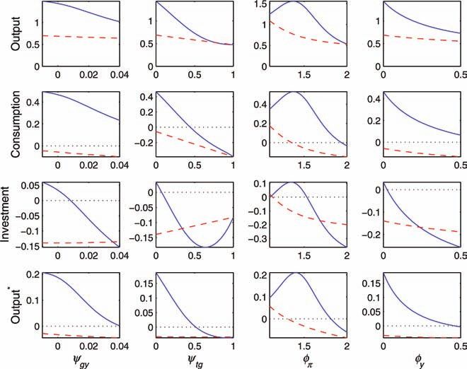
Figure 3. Government Spending Multipliers: Role of
Parameters That Characterize Fiscal and Monetary Policy
Notes: Baseline (solid) vs. debt consolidation through taxes only (dashed).
Multiplier is computed as cumulative change in variable of interest relative
to cumulative change in government spending during first four quarters. For-
eign economy variables are indicated with an asterisk (*). ψ-parameters and
φ-parameters characterize fiscal and monetary rules, respectively.
extensive sensitivity analysis to understand how precisely the trans-
mission mechanism depends on the parameters characterizing the
policy framework, and the deeper economic structures.
A synthesis of our sensitivity exercises is provided in figures 3
and 4. It plots a measure of multipliers computed as the cumulative
response of domestic output, consumption, and investment as well as
foreign output, each scaled by the cumulative rise in domestic gov-
ernment spending during the first four quarters following the initial
impulse. On the horizontal axis we consider a wide range of values for
the parameters of interest. As before, solid lines refer to experiments
conducted under the assumption of spending reversals, and dashed30 International Journal of Central Banking March 2010
lines refer to experiments under the assumption of complete tax
finance. Figure 3 explores the role of parameters that characterize
fiscal and monetary policy.
The first column shows multipliers for different values of ψgy ,
which captures the responsiveness of government spending to the
lagged output gap. A negative (positive) value implies a counter-
cyclical (procyclical) spending rule. We find that procyclicality in
spending tends to reduce multipliers both at home and abroad.
Intuitively, procyclicality triggers additional spending following the
initial exogenous shock, increasing the output gap and thus the mon-
etary policy rate. In a sense, procyclicality works in the opposite
direction than spending reversals.22
The extent of contemporaneous tax finance, ψtg , is considered in
the second column. Results are quite straightforward in this case.
Multipliers are largest in the baseline scenario of complete contem-
poraneous debt finance. For the other extreme, fully front-loaded
tax finance, multipliers are considerably smaller. Quite intuitively,
the mechanism of spending reversals is less consequential, the lower
is the public debt generated by the initial surge in government
spending.
The fiscal transmission mechanism is, furthermore, shaped by the
interaction of monetary and fiscal policies, especially so under spend-
ing reversals, a point already stressed in Corsetti, Meier, and Müller
(2009a). We assess the monetary side of this interaction systemati-
cally in columns 3 and 4, varying the interest rate rule coefficients
φπ and φy . If monetary policy is characterized by a very hawkish
stance—i.e., if these coefficients take high values—multipliers are
smaller. Intuitively, under a hawkish monetary policy rule, the equi-
librium allocation is close to the flexible price allocation, reducing
the scope for output adjustment in response to the shock. Short-
term real rates respond strongly to fiscal policy, making long-term
rates less sensitive to an anticipation of a future contraction in public
demand. Interestingly, however, under spending reversals multipli-
ers and spillovers are non-monotonic in the policymakers’ aversion
to inflation: they tend to fall also when policymakers are relatively
dovish, i.e., for low values of φπ . The reason is that monetary policy
22
Note that we only consider a limited range of values of ψgy , because lower
values would induce indeterminacy of the equilibrium.Vol. 6 No. 1 Cross-Border Spillovers from Fiscal Stimulus 31
Figure 4. Government Spending Multipliers: Role of
Structural Model Features Likely to Impact International
Dimension of Fiscal Transmission Mechanism
Notes: Baseline (solid) vs. debt consolidation through taxes only (dashed). Mul-
tiplier is computed as cumulative change in variable of interest relative to cumu-
lative change in government spending during first four quarters. Foreign economy
variables are indicated with an asterisk (*). σ measures the trade elasticity, is
measures the import-to-GDP ratio in steady state (determined by ωF ), ς meas-
ures the size of the domestic economy on the unit interval, and λ measures the
fraction of rule-of-thumb consumers.
hardly lowers interest rates when lower public spending (the rever-
sal) puts downward pressure on inflation. Because of the interplay
of lower short-term rates on impact and higher rates in the medium
run, long-term real rates fall by less (and private absorption rises by
less) than in the baseline scenario with φπ = 1.5.
The role of structural model features which are likely to impact
the international dimension of the fiscal transmission mechanism are
explored in figure 4. The figure shows how multipliers and spillovers
vary with trade price elasticities, openness, size, and the share of32 International Journal of Central Banking March 2010
non-asset-holding households. Consider first the effects of varying
the trade price elasticity, indexed by the elasticity of substitution
(σ), shown by the graphs in the left column. With spending rever-
sals (the solid lines in the figure), cross-border output spillovers are
stronger for a higher degree of substitutability between domestic
and foreign goods. Intuitively, as the home government claims more
domestic output, it is more tempting for households and firms to
switch to foreign products. Correspondingly, domestic multipliers
for output, consumption, and investment are lower.23
Similarly, when spending increases are entirely matched by (cur-
rent or future) tax hikes (the dashed line), a higher trade elasticity
also reduces domestic spending multipliers for output and consump-
tion, while raising spending spillovers on foreign output. In this case,
however, multipliers and spillovers are much lower, in some cases
negative. Hence, the distance between the solid and the dashed
lines—capturing the role of the debt-stabilizing regime—remains
positive and roughly stable for different values of the trade elasticity.
Analogous considerations apply to the degree of openness of the
economy measured by the import-to-GDP ratio in steady state (sec-
ond column), which is governed by the home bias parameter ωF . In
our experiments we vary the import share between 5 and 40 per-
cent by adjusting the home bias in private absorption accordingly.
To account for the empirical regularity that home bias is stronger in
government spending than in private demand (Corsetti and Müller
2006), we assume throughout that the import content in govern-
ment spending is only half the import share of the entire economy.
We find that the more open the domestic economy, the larger the
foreign output multiplier; external “demand leakages” via higher
imports simultaneously reduce the fiscal transmission on the level
of domestic activity. Note that, relative to the standard experiment,
the differential induced by spending reversals on the foreign output
spillover is actually increasing in the degree of openness.
As a third experiment, we vary home-country size (ς) for a given
degree of openness of the home economy (third column). Increasing
23
We found that the long-term rate actually falls by more for higher values
of σ (not shown). Interestingly, however, a larger fall in long-term rates is not
accompanied by a larger real depreciation as the financial transmission through
foreign interest rates is also more pronounced.You can also read