Deep Reinforcement Learning in Ice Hockey for Context-Aware Player Evaluation
←
→
Page content transcription
If your browser does not render page correctly, please read the page content below
Deep Reinforcement Learning in Ice Hockey
                                                                          for Context-Aware Player Evaluation

                                                                                  Guiliang Liu and Oliver Schulte
                                                                               Simon Fraser University, Burnaby, Canada
                                                                                  gla68@sfu.ca, oschulte@cs.sfu.ca

                                                                  Abstract
arXiv:1805.11088v3 [cs.LG] 16 Jul 2018

                                              A variety of machine learning models have been
                                              proposed to assess the performance of players in
                                              professional sports. However, they have only a lim-
                                              ited ability to model how player performance de-
                                              pends on the game context. This paper proposes a
                                              new approach to capturing game context: we ap-
                                              ply Deep Reinforcement Learning (DRL) to learn
                                              an action-value Q function from 3M play-by-play
                                              events in the National Hockey League (NHL). The
                                              neural network representation integrates both con-           Figure 1: Ice Hockey Rink. Ice hockey is a fast-paced team sport,
                                                                                                           where two teams of skaters must shoot a puck into their opponent’s
                                              tinuous context signals and game history, using a            net to score goals.
                                              possession-based LSTM. The learned Q-function
                                              is used to value players’ actions under different
                                              game contexts. To assess a player’s overall perfor-             Recently, Markov models have been used to address these
                                              mance, we introduce a novel Game Impact Metric               limitations. [Routley and Schulte, 2015] used states of a
                                              (GIM) that aggregates the values of the player’s ac-         Markov Game Model to capture game context and compute
                                              tions. Empirical Evaluation shows GIM is consis-             a Q function, representing the chance that a team scores the
                                              tent throughout a play season, and correlates highly         next goal, for all actions. [Cervone et al., 2014] applied a
                                              with standard success measures and future salary.            competing risk framework with Markov chain to model game
                                                                                                           context, and developed EPV, a point-wise conditional value
                                                                                                           similar to a Q function, for each action . The Q-function con-
                                         1   Introduction: Valuing Actions and Players                     cept offers two key advantages for assigning values to actions
                                         With the advancement of high frequency optical tracking           [Schulte et al., 2017a; Decroos et al., 2018]: 1) All actions are
                                         and object detection systems, more and larger event stream        scored on the same scale by looking ahead to expected out-
                                         datasets for sports matches have become available. There          comes. 2) Action values reflect the match context in which
                                         is increasing opportunity for large-scale machine learning to     they occur. For example, a late check near the opponent’s
                                         model complex sports dynamics. Player evaluation is a ma-         goal generates different scoring chances than a check at other
                                         jor task for sports modeling that draws attention from both       locations and times.
                                         fans and team managers, who want to know which players to            The states in the previous Markov models represent only a
                                         draft, sign or trade. Many models have been proposed [But-        partial game context in the real sports match, but nonethe-
                                         trey et al., 2011; Macdonald, 2011; Decroos et al., 2018;         less the models assume full observability. Also, they pre-
                                         Kaplan et al., 2014]. The most common approach has been to        discretized input features, which leads to loss of information.
                                         quantify the value of a player’s action, and to evaluate play-    In this work, we utilize a deep reinforcement learning (DRL)
                                         ers by the total value of the actions they took [Schuckers and    model to learn an action-value Q function for capturing the
                                         Curro, 2013; McHale et al., 2012].                                current match context. The neural network representation
                                            However, traditional sports models assess only the actions     can easily incorporate continuous quantities like rink loca-
                                         that have immediate impact on goals (e.g. shots), but not the     tion and game time. To handle partial observability, we intro-
                                         actions that lead up to them (e.g. pass, reception). And action   duce a possession-based Long Short Term Memory (LSTM)
                                         values are assigned taking into account only a limited context    architecture that takes into account the current play history.
                                         of the action. But in realistic professional sports, the rele-    Unlike most previous work on active reinforcement learn-
                                         vant context is very complex, including game time, position       ing (RL), which aims to compute optimal strategies for com-
                                         of players, score and manpower differential, etc.                 plex continuous-flow games [Hausknecht and Stone, 2015;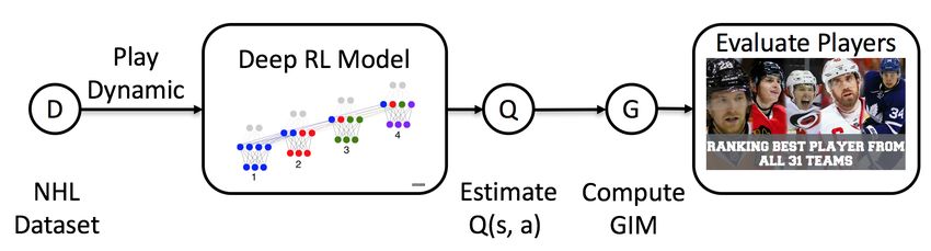
Mnih et al., 2015], we solve a prediction (not control) prob-        dynamic game tracking data, we apply Reinforcement Learn-
lem in the passive learning (on policy) setting [Sutton and          ing to estimate the action value function Q(s, a), which as-
Barto, 1998]. We use RL as a behavioral analytics tool for           signs a value to action a given game state s. We define a new
real human agents, not to control artificial agents.                 player evaluation metric called Goal Impact Metric (GIM)
   Given a Q-function, the impact of an action is the change         to value each player, based on the aggregated impact of their
in Q-value due to the action. Our novel Goal Impact Met-             actions, which is defined in Section 6 below. Player evalua-
ric (GIM) aggregates the impact of all actions of a player.          tion is a descriptive task rather than a predictive generaliza-
To our knowledge, this is the first player evaluation metric         tion problem.As game event data does not provide a ground
based on DRL. The GIM metric measures both players’ of-              truth rating of player performance, our experiments assess
fensive and defensive contribution to goal scoring. For player       player evaluation as an unsupervised problem in Section 7.
evaluation, similar to clustering, ground truth is not avail-
able. A common methodology [Routley and Schulte, 2015;
Pettigrew, 2015] is to assess the predictive value of a player
evaluation metric for standard measures of success. Empiri-
cal comparison between 7 player evaluation metrics finds that
1) given a complete season, GIM correlates the most with 12
standard success measures and is the most temporally consis-
tent metric, 2) given partial game information, GIM general-
izes best to future salary and season total success.                            Figure 2: System Flow for Player Evaluation

2   Related Work                                                     4   Play Dynamic in NHL
We discuss the previous work most related to our approach.           We utilize a dataset constructed by SPORTLOGiQ using
   Deep Reinforcement Learning. Previous DRL work has                computer vision techniques. The data provide information
focused on control in continuous-flow games, not predic-             about game events and player actions for the entire 2015-
tion [Mnih et al., 2015]. Among these papers, [Hausknecht            2016 NHL (largest professional ice hockey league) season,
and Stone, 2015] use a very similar network architecture to          which contains 3,382,129 events, covering 30 teams, 1140
ours, but with a fixed trace length parameter rather than our        games and 2,233 players. Table 1 shows an excerpt. The data
possession-based method. Hausknecht and Stone find that for          track events around the puck, and record the identity and ac-
partially observable control problems, the LSTM mechanism            tions of the player in possession, with space and time stamps,
outperforms a memory window. Our study confirms this find-           and features of the game context. The table utilizes adjusted
ing in an on policy prediction problem.                              spatial coordinates where negative numbers refer to the de-
   Player Evaluation. Albert et al. 2017 provide several up-         fensive zone of the acting player, positive numbers to his of-
to-date survey articles about evaluating players. A funda-           fensive zone. Adjusted X-coordinates run from -100 to +100,
mental difficulty for action value counts in continuous-flow         Y-coordinates from 42.5 to -42.5, and the origin is at the ice
games is that they traditionally have been restricted to goals       center as in Figure 1. We augment the data with derived fea-
and actions immediately related to goals (e.g. shots). The           tures in Table 2 and list the complete feature set in Table 3.
Q-function solves this problem by using lookahead to assign             We apply the Markov Game framework [Littman, 1994]
values to all actions.                                               to learn an action value function for NHL play. Our nota-
   Player Evaluation with Reinforcement Learning. Using              tion for RL concepts follows [Mnih et al., 2015]. There are
the Q-function to evaluate players is a recent development           two agents Home resp. Away representing the home resp.
[Schulte et al., 2017a; Cervone et al., 2014; Routley and            away team. The reward, represented by goal vector gt is
Schulte, 2015]. Schulte et al. discretized location and time         a 1-of-3 indicator vector that specifies which team scores
coordinates and applied dynamic programming to learn a Q-            (Home, Away, Neither ). An action at is one of 13 types,
function. Discretization leads to loss of information, unde-         including shot, block, assist, etc., together with a mark that
sirable spatio-temporal discontinuities in the Q-function, and       specifies the team executing the action, e.g. Shot(Home).
generalizes poorly to unobserved parts of the state space. For       An observation is a feature vector xt for discrete time step
basketball, Cervone et al. defined a player performance met-         t that specifies a value for the 10 features listed in Table 3.
ric based on an expected point value model that is equivalent        We use the complete sequence st ≡ (xt , at−1 , xt−1 , . . . , x0 )
to a Q-function. Their approach assumes complete observ-             as the state representation at time step t [Mnih et al., 2015],
ability (of all players at all times), while our data provide par-   which satisfies the Markov property.
tial observability only.                                                We divide NHL games into goal-scoring episodes, so that
                                                                     each episode 1) begins at the beginning of the game, or
3   Task Formulation and Approach                                    immediately after a goal, and 2) terminates with a goal or
                                                                     the end of the game. A Q function represents the condi-
Player evaluation (the “Moneyball” problem) is one of the            tional probability of the event that the home resp. away team
most studied tasks in sports analytics. Players are rated by         scores the goal at the end of the current episode (denoted
their observed performance over a set of games. Our ap-              goal Home = 1 resp. goal Away = 1 ), or neither team does
proach to evaluating players is illustrated in Figure 2. Given       (denoted goal Neither = 1 ):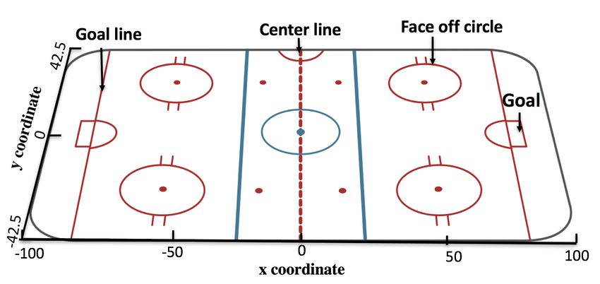
GID=GameId, PID=playerId, GT=GameTime, TID=TeamId, MP=Manpower, GD=Goal Difference, OC = Outcome, S=Succeed, F=Fail, P
   = Team Possess puck, H=Home, A=Away, H/A=Team who performs action, TR = Time Remain, PN = Play Number, D = Duration
    GID     PID   GT      TID       X       Y       MP       GD     Action   OC     P        Velocity        TR        D    Angle     H/A   PN
    1365    126   14.3      6     -11.0    25.5     Even      0      Lpr      S     A      (-23.4, 1.5)     3585.7    3.4   0.250      A     4
    1365    126   17.5      6     -23.5   -36.5     Even      0     Carry     S     A      (-4.0, -3.5)     3582.5    3.1   0.314      A     4
    1365    270   17.8     23      14.5    35.5     Even      0     Block     S     A     (-27.0, -3.0)     3582.2    0.3   0.445      H     4
    1365    126   17.8      6     -18.5   -37.0     Even      0      Pass     F     A         (0, 0)        3582.2    0.0   0.331      A     4
    1365    609   19.3     23     -28.0    25.5     Even      0      Lpr      S     H     (-30.3, -7.5)     3580.6    1.5   0.214      H     5
    1365    609   19.3     23     -28.0    25.5     Even      0      Pass     S     H         (0,0)         3580.6    0.0   0.214      H     5

                                Table 1: Dataset Example                                                  Table 2: Derived Features

               Name                  Type                 Range
       X Coordinate of Puck        Continuous          [-100, 100]
       Y Coordinate of Puck        Continuous         [-42.5, 42.5]
          Velocity of Puck         Continuous          (-inf, +inf)
        Game Time Remain           Continuous           [0, 3600]
         Score Differential         Discrete           (-inf, +inf)
       Manpower Situation           Discrete         {EV, SH, PP}
          Event Duration           Continuous            [0, +inf)
          Action Outcome            Discrete      {successful, failure}
    Angle between puck and goal    Continuous        [−3.14, 3.14]
       Home or Away Team            Discrete        {Home, Away}

                   Table 3: Complete Feature List

        Qteam (s, a) = P (goal team = 1 |st = s, at = a)

   where team is a placeholder for one of                                    Figure 3: Our design is a 5-layer network with 3 hidden layers.
Home, Away, Neither . This Q-function represents the                         Each hidden layer contains 1000 nodes, which utilize a relu acti-
probability that a team scores the next goal, given current                  vation function. The first hidden layer is the LSTM layer, the re-
                                                                             maining layers are fully connected. Temporal-difference learning
play dynamics in the NHL (cf. Schulte et al.; Routley
                                                                             looks ahead to the next goal, and the LSTM memory traces back to
and Schulte). Different Q-functions for different expected                   the beginning of the play (the last possession change).
outcomes have been used to capture different aspects of
NHL play dynamics, such as match win [Pettigrew, 2015;
Kaplan et al., 2014; Routley and Schulte, 2015] and penalties                5.1   Network Architecture
[Routley and Schulte, 2015]. For player evaluation, the
next-goal Q function has three advantages. 1) The next-goal                  Figure 3 shows our model structure. Three output nodes
reward captures what a coach expects from a player. For                      represent the estimates Q̂Home (s, a), Q̂Away (s, a) and
example, if a team is ahead by two goals with one minute
                                                                             Q̂Neither (s, a). Output values are normalized to probabilities.
left in the match, a player’s actions have negligible effect
on final match outcome. Nonetheless professionals should                     The Q̂-functions for each team share weights. The network
keep playing as well as they can and maximize the scoring                    architecture is a Dynamic LSTM that takes as inputs a current
chances for their own team. 2) The Q-values are easy to                      sequence st , an action at and a dynamic trace length tl t .1
interpret, since they model the probability of an event that
is a relatively short time away (compared to final match                     5.2   Weight Training
outcome). 3) Increasing the probability that a player’s team
scores the next goal captures both offensive and defensive                   We apply an on-policy Temporal Difference (TD) predic-
value. For example, a defensive action like blocking a shot                  tion method Sarsa [Sutton and Barto, 1998, Ch.6.4], to es-
decreases the probability that the other team will score the                 timate Qteam (s, a) for the NLH play dynamics observed in
next goal, thereby increasing the probability that the player’s              our dataset. Weights θ are optimized by minibatch gradient
own team will score the next goal.                                           descent via backpropagation. We used batch size 32 (deter-
                                                                             mined experimentally). The Sarsa gradient descent update at
                                                                             time step t is based on a squared-error loss function:
5     Learning Q values with DP-LSTM Sarsa
We take a function approximation approach and learn a neural                     1
                                                                                   We experimented with a single-hidden layer, but weight training
network that represents the Q-function (Qteam (s, a)).                       failed to converge.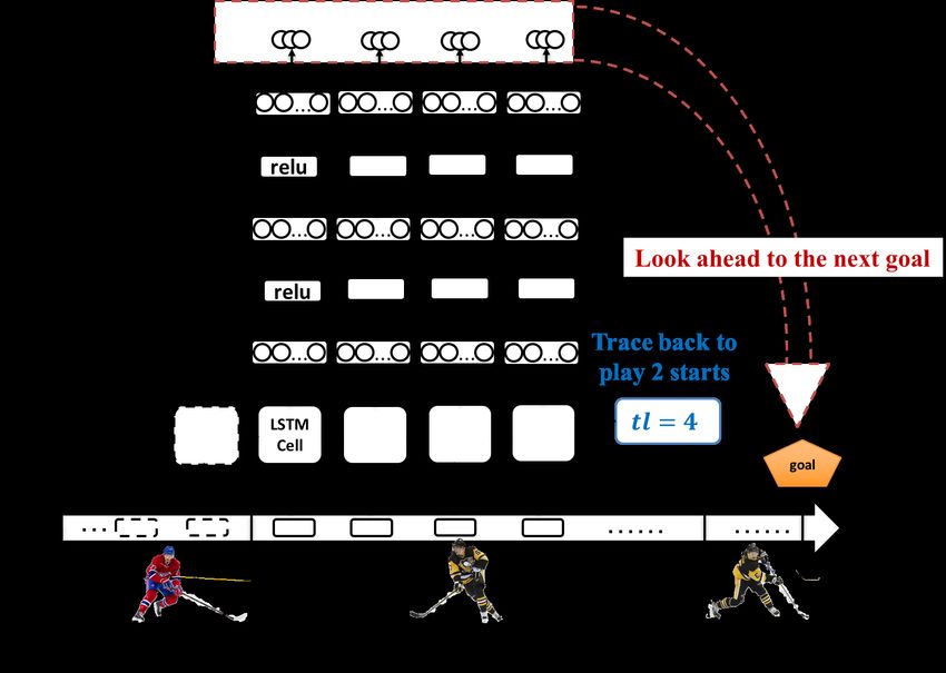
6 Player Evaluation
In this section, we define our novel Goal Impact Metric and
give an example player ranking.
6.1 Player Evaluation Metric
Our Q-function concept provides a novel AI-based defini-
tion for assigning a value to an action. Like [Schulte et al.,
2017b], we measure the quality of an action by how much it
changes the expected return of a player’s team. Whereas the
scoring chance at a time measures the value of a state, and
therefore depends on the previous efforts of the entire team,
the change in value measures directly the impact of an action
by a specific player. In terms of the Q-function, this is the
change in Q-value due to a player’s action. This quantity is
defined as the action’s impact. The impact can be visualized
as the difference between successive points in the Q-value
ticker (Figure 4). For our specific choice of Next Goal as the
reward function, we refer to goal impact. The total impact
of a player’s actions is his Goal Impact Metric (GIM). The
formal equations are:
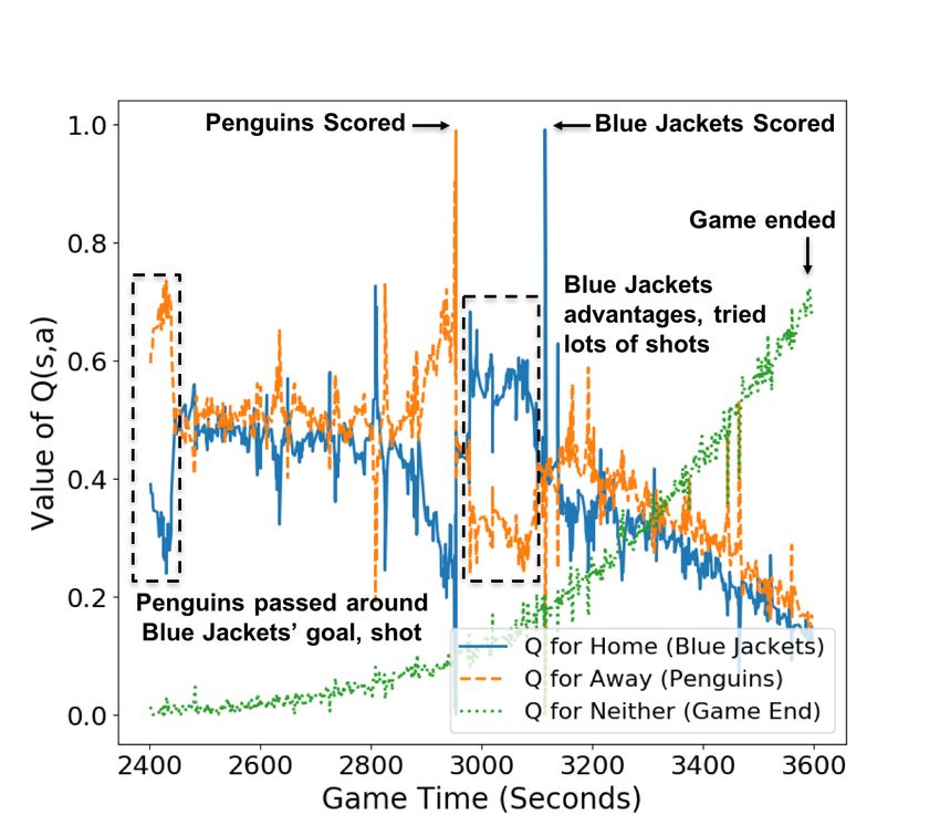
Figure 4: Temporal Projection of the method. For each team, and
each game time, the graph shows the chance the that team scores impact team (st , at ) = Qteam (st , at ) − Qteam (st−1 , at−1 )
the next goal, as estimated by the model. Major events lead to major X
changes in scoring chances, as annotated. The network also captures GIM i (D) = niD (s, a) × impact team i (s, a)
smaller changes associated with every action under different game s,a
contexts.
where D indicates our dataset, team i denotes the team of
player i, and niD (s, a) is the number of times that player i
was observed to perform action a at s. Because it is the sum
of differences between subsequent Q values, the GIM metric
Lt (θt ) = E[(gt + Q̂(st+1 , at+1 , θt ) − Q̂(st , at , θt ))2 ] inherits context-sensitivity from the Q function.
θt+1 = θt + α∇θ L(θt )
6.2 Rank Players with GIM
where g and Q̂ are for a single team. LSTM training re- Table 4 lists the top-20 highest impacts players, with basic
quires setting a trace length tl t parameter. This key param- statistics. All these players are well-known NHL stars. Tay-
eter controls how far back in time the LSTM propagates the lor Hall tops the ranking although he did not score the most
error signal from the current time at the input history. Team goals. This shows how our ranking, while correlated with
sports like Ice Hockey show a turn-taking aspect where one goals, also reflects the value of other actions by the player.
team is on the offensive and the other defends; one such turn For instance, we find that the total number of passes per-
is called a play. We set tl t to the number of time steps from formed by Taylor Hall is exceptionally high at 320. Our met-
current time t to the beginning of the current play (with a ric can be used to identify undervalued players. For instance,
maximum of 10 steps). A play ends when the possession Johnny Gaudreau and Mark Scheifele drew salaries below
of puck changes from one team to another. Using posses- what their GIM rank would suggest. Later they received a
sion changes as break points for temporal models is common $5M + contract for the 2016-17 season.
in several continuous-flow sports, especially basketball [Cer-
vone et al., 2014; Omidiran, 2011]. We apply Tensorflow to
implement training; our source code is published on-line.2
7 Empirical Evaluation
Illustration of Temporal Projection. Figure 4 shows a value We describe our comparison methods and evaluation method-
ticker [Decroos et al., 2017; Cervone et al., 2014] that repre- ology. Similar to clustering problems, there is no ground truth
sents the evolution of the Q function from the 3rd period of for the task of player evaluation. To assess a player evaluation
a match between the Blue Jackets (Home team) and the Pen- metric, we follow previous work [Routley and Schulte, 2015;
guins (Away team), Nov. 17, 2015. The figure plots values Pettigrew, 2015] and compute its correlation with statistics
of the three output nodes. We highlight critical events and that directly measure success like Goals, Assists, Points, Play
match contexts to show the context-sensitivity of the Q func- Time (Section 7.2). There are two justifications for compar-
tion. High scoring probabilities for one team decrease those ing with success measures. (1) These statistics are generally
of its opponent. The probability that neither team scores rises recognized as important measures of a player’s strength, be-
significantly at the end of the match. cause they indicate the player’s ability to contribute to game-
changing events. So a comprehensive performance metric
2
https://github.com/Guiliang/DRL-ice-hockey ought to be related to them. (2) The success measures are
Name          GIM     Assists   Goals   Points   Team      Salary     the model has been trained off-line, the GIM metric can be
      Taylor Hall     96.40     39       26      65      EDM     $6,000,000
     Joe Pavelski     94.56     40       38      78       SJS    $6,000,000   computed quickly with a single pass over the data.
  Johnny Gaudreau     94.51     48       30       78     CGY      $925,000       Significance Test. To assess whether GIM is significantly
     Anze Kopitar     94.10     49       25      74      LAK    $7,700,000
    Erik Karlsson     92.41     66       16       82     OTT    $7,000,000    different from the other player evaluation metrics, we per-
  Patrice Bergeron    92.06     36       32       68     BOS    $8,750,000    form paired t-tests over all players. The null hypothesis is
   Mark Scheifele     90.67     32       29       61     WPG      $832,500    rejected with respective p-values: 1.1 ∗ 10−186 , 7.6 ∗ 10−204 ,
    Sidney Crosby     90.21     49       36      85       PIT   $12,000,000
    Claude Giroux     89.64     45       22      67       PHI   $9,000,000    8 ∗ 10−218 , 3.9 ∗ 10−181 , 4.7 ∗ 10−201 and 1.3 ∗ 10−05 for
  Dustin Byfuglien    89.46     34       19       53     WPG    $6,000,000    PlusMinus, GAR, WAR, EG, SI and GIM-T1, which shows
     Jamie Benn       88.38     48       41       89     DAL     $5,750,000
     Patrick Kane     87.81     60       46      106     CHI    $13,800,000
                                                                              that GIM values are very different from other metrics’ values.
     Mark Stone       86.42     38       23      61      OTT    $2,250,000
    Blake Wheeler     85.83     52       26      78      WPG    $5,800,000    7.2   Season Totals: Correlations with standard
     Tyler Toffoli    83.25     27       31      58      DAL    $2,600,000
    Charlie Coyle     81.50     21       21       42     MIN    $1,900,000
                                                                                    Success Measures
     Tyson Barrie     81.46    36        13       49     COL    $3,200,000    In the following experiment, we compute the correlation be-
   Jonathan Toews     80.92     30       28      58      CHI    $13,800,000
    Sean Monahan      80.92    36        27       63     CGY      $925,000    tween player ranking metrics and success measures over the
 Vladimir Tarasenko   80.68     34       40      74      STL    $8,000,000    entire season. Table 5 shows the correlation coefficients of
                                                                              the comparison methods with 14 standard success measures:
         Table 4: 2015-2016 Top-20 Player Impact Scores                       Assist, Goal, Game Wining Goal (GWG), Overtime Goal
                                                                              (OTG), Short-handed Goal (SHG), Power-play Goal (PPG),
                                                                              Shots (S), Point, Short-handed Point (SHP), Power-play Point
often forecasting targets for hockey stakeholders, so a good                  (PPP), Face-off Win Percentage (FOW), Points Per Game
player evaluation metric should have predictive value for                     (P/GP), Time On Ice (TOI) and Penalty Minute (PIM). These
them. For example, teams would want to know how many                          are all commonly used measures available from the NHL of-
points an offensive player will contribute. To evaluate the                   ficial website (www.nhl.com/stats/player). GIM achieves the
ability of the GIM metric for generalizing from past perfor-                  highest correlation in 12 out of 14 success measures. For
mance to future success, we report two measurements: How                      the remaining two (TOI and PIM), GIM is comparable to
well the GIM metric predicts a total season success measure                   the highest. Together, the Q-based metrics GIM, GIM-1 and
from a sample of matches only (Section 7.3), and how well                     SI show the highest correlations with success measures. EG
the GIM metric predicts the future salary of a player in subse-               is only the fourth best metric, because it considers only the
quent seasons (Section 7.4). Mapping performance to salaries                  expected value of shots without look-ahead. The traditional
is a practically important task because it provides an objective              sports analytics metrics correlate poorly with almost all suc-
standard to guide players and teams in salary negotiations [Id-               cess measures. This is evidence that AI techniques that pro-
son and Kahane, 2000].                                                        vide fine-grained expected action value estimates lead to bet-
                                                                              ter performance metrics. With the neural network model,
7.1   Comparison Player Evaluation Metrics                                    GIM can handle continuous input without pre-discretization.
We compare GIM with the following player evaluation met-                      This prevents the loss of game context information and ex-
rics to show the advantage of 1) modeling game context 2)                     plains why both GIM and GIM-T1 performs better than SI in
incorporating continuous context signal 3) including history.                 most success measures. And the higher correlation of GIM
   Our first baseline method Plus-Minus (+/-) is a commonly                   compared to GIM-T1 also demonstrates the value of game
used metric that measures how the presence of a player in-                    history. In terms of absolute correlations, GIM achieves high
fluences the goals of his team [Macdonald, 2011]. The sec-                    values, except for the very rare events OTG, SHG, SHP and
ond baseline method Goal-Above-Replacement (GAR) esti-                        FOW. Another exception is Penalty Minutes (PIM), which in-
mates the difference of team’s scoring chances when the tar-                  terestingly, show positive correlation with all player evalua-
get player plays, vs. replacing him or her with an average                    tion metrics, although penalties are undesirable. We hypoth-
player [Gerstenberg et al., 2014]. Win-Above-Replacement                      esize that better players are more likely to receive penalties,
(WAR), our third baseline method, is the same as GAR but                      because they play more often and more aggressively.
for winning chances [Gerstenberg et al., 2014]. Our fourth
baseline method Expected Goal (EG) weights each shot                          7.3   Round-by-Round Correlations: Predicting
by the chance of it leading to a goal. These four meth-                             Future Performance From Past Performance
ods consider only very limited game context. The last base-                   A sports season is commonly divided into rounds. In round
line method Scoring Impact (SI) is the most similar method                    n, a team or player has finished n games in a season. For
to GIM based on Q-values. But Q-values are learned with                       a given performance metric, we measure the correlation be-
pre-discretized spatial regions and game time [Schulte et al.,                tween (i) its value computed over the first n rounds, and (ii)
2017a]. As a lesion method, we include GIM-T1, where we                       the value of the three main success measures, assists, goals,
set the maximum trace length of LSTM to 1 (instead of 10)                     and points, computed over the entire season. This allows
in computing GIM. This comparison assesses the importance                     us to assess how quickly different metrics acquire predictive
of including enough history information.                                      power for the final season total, so that future performance
   Computing Cost. Compared to traditional metrics like +/-,                  can be predicted from past performance. We also evaluate
learning a Q-function is computationally demanding (over 5                    the auto-correlation of a metric’s round-by-round total with
million gradient descent steps on our dataset). However, after                its own season total. The auto-correlation is a measure of
methods   Assist   Goal    GWG     OTG      SHG     PPG       S
   +/-     0.236    0.204   0.217    0.16    0.095   0.099   0.118
  GAR      0.527    0.633   0.552   0.324    0.191   0.583   0.549
  WAR      0.516    0.652   0.551   0.332    0.192   0.564   0.532
   EG      0.783    0.834   0.704   0.448    0.249   0.684   0.891
   SI      0.869    0.745   0.631   0.411     0.27   0.591   0.898
 GIM-T1    0.873    0.752   0.682   0.428    0.291   0.607   0.877
  GIM      0.875    0.878   0.751   0.465    0.345    0.71   0.912

 methods   Point    SHP      PPP     FOW     P/GP     TOI    PIM
   +/-     0.237    0.159   0.089   -0.045   0.238   0.141   0.049
  GAR      0.622    0.226   0.532     0.16   0.616   0.323   0.089
  WAR      0.612    0.235   0.531    0.153   0.605   0.331   0.078
   EG      0.854    0.287   0.729    0.28    0.702   0.722   0.354
   SI      0.869     0.37   0.707   0.185    0.655   0.955   0.492
 GIM-T1    0.902    0.384   0.736   0.288    0.738   0.777   0.347
  GIM       0.93    0.399   0.774    0.295   0.749   0.835   0.405

      Table 5: Correlation with standard success measures.

temporal consistency, which is a desirable feature [Pettigrew,
2015], because generally the skill of a player does not change
greatly throughout a season. Therefore a good performance
metric should show temporal consistency.
   We focused on the expected value metrics EG, SI, GIM-T1
                                                                     Figure 5: Correlations between round-by-round metrics and season
and GIM, which had the highest correlations with success in          totals.
Table 5. Figure 5 shows metrics’ round-by-round correlation
coefficients with assists, goals, and points. The bottom right                methods     2016 to 2017 Season   2017 to 2018 Season
shows the auto-correlation of a metric’s round-by-round total                Plus Minus          0.177                 0.225
with its own season total. GIM is the most stable metric as                     GAR              0.328                 0.372
measured by auto-correlation: after half the season, the cor-                   WAR              0.328                 0.372
                                                                                 EG              0.587                   0.6
relation between the round-by-round GIM and the final GIM                        SI              0.609                 0.668
is already above 0.9.                                                         GIM-T1             0.596                  0.69
   We find both GIM and GIM-T1 eventually dominate                              GIM              0.666                 0.763
the predictive value of the other metrics, which shows the
advantages of modeling sports game context without pre-                         Table 6: Correlation with Players’ Contract
discretization. And possession-based GIM also dominates
GIM-T1 after the first season half, which shows the value of         players in the right bottom part, with high GIM but low salary
including play history in the game context. But how quickly          in their new contract. It is interesting that the percentage of
and how much the GIM metrics improve depends on the                  players who are undervalued in their new contract decreases
specific success measure. For instance, in Figure 5, GIM’s           in the next season (from 32/258 in 2016-17 season to 8/125
round-by-round correlation with Goal (top right graph) dom-          in 2017-2018 season). This suggests that GIM provides an
inates by round 10, while others require a longer time.              early signal of a player’s value after one season, while it often
                                                                     takes teams an additional season to recognize performance
7.4   Future Seasons: Predicting Players’ Salary                     enough to award a higher salary.
In professional sports, a team will give a comprehensive eval-
uation to players before deciding their contract. The more
value players provide, the larger contract they will get. Ac-
                                                                     8   Conclusion and Future Work
cordingly, a good performance metric should be positively re-        We investigated Deep Reinforcement Learning (DRL) for
lated to the amount of players’ future contract. The NHL reg-        professional sports analytics. We applied DRL to learn
ulates when players can renegotiate their contracts, so we fo-       complex spatio-temporal NHL dynamics. The trained neural
cus on players receiving a new contract following the games          network provides a rich source of knowledge about how a
in our dataset (2015-2016 season).                                   team’s chance of scoring the next goal depends on the match
   Table 6 shows the metrics’ correlations with the amount           context. Based on the learned action values, we developed
of players’ contract over all the players who obtained a new         an innovative context-aware performance metric GIM that
contract during the 2016-17 and 2017-18 NHL seasons. Our             provides a comprehensive evaluation of NHL players, taking
GIM score achieves the highest correlation in both seasons.          into account all of their actions. In our experiments, GIM had
This means that the metric can serve as an objective basis for       the highest correlation with most standard success measures,
contract negotiations. The scatter plots of Figure 6 illustrate      was the most temporally consistent metric, and generalized
GIM’s correlation with amount of players’ future contract.           best to players’ future salary. Our approach applies to similar
In the 2016-17 season (left), we find many underestimated            continuous-flow sports games with rich game contexts,
[Idson and Kahane, 2000] Todd L Idson and Leo H Kahane.
                                                                    Team effects on compensation: an application to salary
                                                                    determination in the National Hockey League. Economic
                                                                    Inquiry, 38(2):345–357, 2000.
                                                                 [Kaplan et al., 2014] Edward H Kaplan, Kevin Mongeon,
                                                                    and John T Ryan. A Markov model for hockey: Man-
                                                                    power differential and win probability added. INFOR: In-
                                                                    formation Systems and Operational Research, 52(2):39–
                                                                    50, 2014.
                                                                 [Littman, 1994] Michael L Littman. Markov games as a
                                                                    framework for multi-agent reinforcement learning. In Pro-
Figure 6: Player GIM vs. Value of new contracts in the 2016-17      ceedings International Conference on Machine Learning,
(left) and 2017-18 (right) NHL season.                              volume 157, pages 157–163, 1994.
                                                                 [Macdonald, 2011] Brian Macdonald. A regression-based
like soccer and basketball. A limitation of our approach is         adjusted plus-minus statistic for NHL players. Journal of
that players get credit only for recorded individual actions.       Quantitative Analysis in Sports, 7(3):29, 2011.
An influential approach to extend credit to all players on       [McHale et al., 2012] Ian G McHale, Philip A Scarf, and
the rink has been based on regression [Macdonald, 2011;             David E Folker.        On the development of a soccer
Thomas et al., 2013]. A promising direction for future work         player performance rating system for the English Premier
is to combine Q-values with regression.                             League. Interfaces, 42(4):339–351, 2012.
                                                                 [Mnih et al., 2015] Volodymyr Mnih, Koray Kavukcuoglu,
                                                                    David Silver, et al. Human-level control through deep re-
Acknowledgements                                                    inforcement learning. Nature, 518(7540):529–533, 2015.
This work was supported by an Engage Grant from the Na-          [Omidiran, 2011] Dapo Omidiran. A new look at adjusted
tional Sciences and Engineering Council of Canada, and a            plus/minus for basketball analysis. In MIT Sloan Sports
GPU donation from NVIDIA Corporation.                               Analytics Conference [online], 2011.
                                                                 [Pettigrew, 2015] Stephen Pettigrew. Assessing the offensive
References                                                          productivity of NHL players using in-game win probabili-
[Albert et al., 2017] Jim Albert, Mark E Glickman, Tim B            ties. In MIT Sloan Sports Analytics Conference, 2015.
  Swartz, and Ruud H Koning. Handbook of Statistical             [Routley and Schulte, 2015] Kurt Routley and Oliver
  Methods and Analyses in Sports. CRC Press, 2017.                  Schulte. A Markov game model for valuing player actions
[Buttrey et al., 2011] Samuel Buttrey, Alan Washburn, and           in ice hockey. In Proceedings Uncertainty in Artificial
  Wilson Price. Estimating NHL scoring rates. Journal of            Intelligence (UAI), pages 782–791, 2015.
  Quantitative Analysis in Sports, 7(3), 2011.                   [Schuckers and Curro, 2013] Michael Schuckers and James
[Cervone et al., 2014] Dan Cervone, Alexander D’Amour,              Curro. Total hockey rating (THoR): A comprehensive
  Luke Bornn, and Kirk Goldsberry. Pointwise: Predicting            statistical rating of national hockey league forwards and
  points and valuing decisions in real time with NBA optical        defensemen based upon all on-ice events. In MIT Sloan
  tracking data. In MIT Sloan Sports Analytics Conference,          Sports Analytics Conference, 2013.
  2014.                                                          [Schulte et al., 2017a] Oliver Schulte, Mahmoud Khademi,
[Decroos et al., 2017] Tom Decroos, Vladimir Dzyuba,                Sajjad Gholami, et al. A Markov game model for valuing
  Jan Van Haaren, and Jesse Davis. Predicting soccer high-          actions, locations, and team performance in ice hockey.
  lights from spatio-temporal match event streams. In AAAI          Data Mining and Knowledge Discovery, pages 1–23,
  2017, pages 1302–1308, 2017.                                      2017.
[Decroos et al., 2018] Tom Decroos, Lotte Bransen, Jan           [Schulte et al., 2017b] Oliver Schulte, Zeyu Zhao, Mehrsan
  Van Haaren, and Jesse Davis. Actions speak louder than            Javan, and Philippe Desaulniers. Apples-to-apples: Clus-
  goals: Valuing player actions in soccer. arXiv preprint           tering and ranking NHL players using location informa-
  arXiv:1802.07127, 2018.                                           tion and scoring impact. In MIT Sloan Sports Analytics
                                                                    Conference, 2017.
[Gerstenberg et al., 2014] Tobias Gerstenberg, Tomer Ull-
                                                                 [Sutton and Barto, 1998] Richard S Sutton and Andrew G
  man, Max Kleiman-Weiner, David Lagnado, and Josh
  Tenenbaum. Wins above replacement: Responsibility at-             Barto. Introduction to reinforcement learning, volume
  tributions as counterfactual replacements. In Proceedings         135. MIT Press Cambridge, 1998.
  of the Cognitive Science Society, volume 36, 2014.             [Thomas et al., 2013] A.C. Thomas, S.L. Ventura, S. Jensen,
[Hausknecht and Stone, 2015] Matthew Hausknecht and Pe-             and S. Ma. Competing process hazard function models
  ter Stone. Deep recurrent Q-learning for partially observ-        for player ratings in ice hockey. The Annals of Applied
  able MDPs. CoRR, abs/1507.06527, 2015.                            Statistics, 7(3):1497–1524, 2013.
You can also read