Degrees of Poverty: The Relationship between Family Income Background and the Returns to Education

Upjohn Institute Working Papers                                                                             Upjohn Research home page

2018

Degrees of Poverty: The Relationship between
Family Income Background and the Returns to
Education
Timothy J. Bartik
W.E. Upjohn Institute, bartik@upjohn.org

Brad J. Hershbein
W.E. Upjohn Institute, hershbein@upjohn.org

Upjohn Institute working paper ; 18-284

Citation
Bartik, Timothy J., and Brad Hershbein. 2018. "Degrees of Poverty: The Relationship between Family Income Background and the
Returns to Education." Upjohn Institute Working Paper 18-284. Kalamazoo, MI: W.E. Upjohn Institute for Employment Research.
https://doi.org/10.17848/wp18-284

This title is brought to you by the Upjohn Institute. For more information, please contact ir@upjohn.org.

Degrees of Poverty: The Relationship between Family Income
                     Background and the Returns to Education
                                  Upjohn Institute Working Paper 18-284

                                          Timothy J. Bartik
                                      email: bartik@upjohn.org
                            W.E. Upjohn Institute for Employment Research

                                           Brad Hershbein
                                    email: Hershbein@upjohn.org
                            W.E. Upjohn Institute for Employment Research

                                                 March 2018

                                                 ABSTRACT

        Drawing on the Panel Study of Income Dynamics, we document a startling empirical
pattern: the career earnings premium from a four-year college degree (relative to a high school
diploma) for persons from low-income backgrounds is considerably less than it is for those from
higher-income backgrounds. For individuals whose family income in high school was above 1.85
times the poverty level, we estimate that career earnings for bachelor’s graduates are 136 percent
higher than earnings for those whose education stopped at high school. However, for individuals
whose family income during high school was below 1.85 times the poverty level, the career
earnings of bachelor’s graduates are only 71 percent higher than those of high school graduates.
This lower premium amounts to $300,000 less in career earnings in present discounted value. We
establish the prevalence and robustness of these differential returns to education across race and
gender, finding that they are driven by whites and men and by differential access to the right tail
of the earnings distribution.

JEL Codes: I24, I26, J24, J31

Key Words: inequality, return to education, career earnings profile, PSID, low-income

Acknowledgments:

       We are grateful to Sarah Hamersma, Michael Hout, Melissa Kearney, Yulya
Truskinovsky, and seminar participants at the 2017 PAA meetings, 2017 APPAM meetings,
2017 SEA meetings, Notre Dame, and the University of Michigan. We thank Wei-Jang Huang
and Nathan Sotherland for excellent research assistance with the PSID. All errors are our own.

Upjohn Institute working papers are meant to stimulate discussion and criticism among the policy research
community. Content and opinions are the sole responsibility of the author.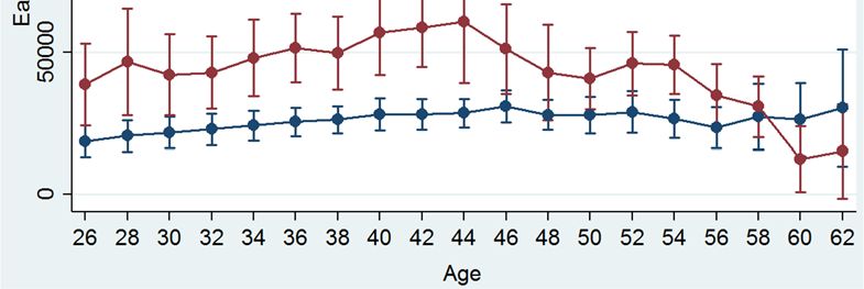

Growing earnings inequality in the United States has been the subject of much research, across a

number of dimensions. This growth is thought to have many causes, ranging from international trade to

technological change to institutional change (e.g., the declining real value of minimum wage, declines in

unionization, and changes in corporate governance), and part of these structural changes have been linked

with rising returns to education. Indeed, a large research literature has sought to describe or explain the

growing gap between the more-educated and less-educated, as well as an increase in earnings dispersion

within the more-educated group (Katz and Murphy 1992; Autor, Katz, Kearney 2006, 2008; Lemieux

2006). The overall growth in earnings inequality, and its relationship with the high (and perhaps still

growing) returns to education, have led to heightened concerns about economic opportunity and mobility.

        The relationship between earnings inequality and returns to education has also led to speculation

among many policymakers and economists that increasing educational attainment, particularly among the

poor, could help equalize economic opportunity, if not outcomes. Although an increase in the share of the

population that is more highly educated would presumably decrease the returns to education through

supply-side factors, possibly stopping or reversing its growth over the past few decades, it is certainly

conceivable that providing more education to the poor might improve their relative earnings outcomes if

not appreciably diminish overall inequality (Hershbein, Kearney, and Summers 2015).

        Yet, another strain of research recognizes that returns to education are heterogeneous for different

groups (Card 1999; Carneiro, Heckman, and Vytlacil 2001, 2011; Brand and Xie 2010), including for

individuals whose parents have different levels of education (Altonji and Dunn 1996) or who vary in

cognitive ability (Ashenfelter and Rouse 1998). This research literature has emphasized the role of

selection in driving unobserved heterogeneity, noting that college attendance and completion vary by

family background (Belley and Lochner 2007; Bailey and Dynarski 2011). Related to this literature are

studies that investigate how child and adolescent experiences—especially poverty—shape career

trajectories (Alexander, Entwhistle, and Olsen 2014). In these studies, a prominent mechanism for the role

                                                      1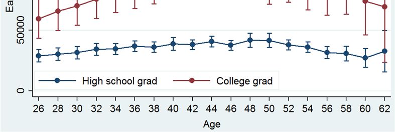

of family socioeconomic background in affecting career earnings is through college attendance and

attainment, with poverty found to be especially harmful for these indicators.

         However, family income background may have career earnings effects well beyond its effect

through college attendance and attainment. Lower-income family background may be associated with

various events and experiences (e.g., family structure and environment, neighborhood influences and peer

influences, school quality) that may lead to lower hard or soft skills or fewer connections, which might in

turn lead to less ability to obtain better jobs. These effects may operate independently from educational

attainment or interact with them heterogeneously. There has been very little work, to our knowledge, on

how childhood poverty (or low family income more generally) affects the return to education, conditional

on achieving it, over the whole career.1 Family income background and educational attainment could

interact because the skills and knowledge obtained through childhood experiences may have

complementarity or substitutability with skills causally imparted by education attainment. For example, if

a higher-family-income background provides better knowledge of social connections and better soft

skills, this may complement better hard skills imparted by the educational system, so that a higher-income

background and higher educational attainment together yield greater earnings returns than either would

yield separately (Deming 2015). Alternatively, perhaps the educational system teaches students from a

low-income background certain soft skills that students from a higher-income background pick up

through other channels, so that school can to some extent substitute for family income background.

Relations of complementarity between family background and educational attainment would lead to

educational returns increasing with higher-income family backgrounds, while relations of substitutability

might lead to educational returns declining with higher-income family backgrounds (Brand and Xie

2010).

         1
          Torche (2011) investigates a related question of how intergenerational mobility varies by
realized education of the children, finding a U-shaped pattern. However, her measures of mobility do not
cover the whole career, and her focus is on absolute mobility rather than heterogeneity in the education
earnings premium, per se.
                                                     2

Furthermore, family income background could correlate with empirically measured returns to

education not due to true causal effects of education, but rather to how family income background affects

who is selected to be educated. For example, low-income students who achieve higher educational

attainment could be positively selected, with only the most motivated and talented succeeding in

overcoming adversity. On the other hand, as policy pushes more low-income students to attain higher

educational credentials, perhaps such marginal students will be negatively selected, with fewer skills.

        In discussing education returns, and how they vary with family income background, we must be

careful in distinguishing between different types of inequality. In the most extreme case, one might hope

that although lower family-income background may handicap earnings prospects for individuals with less

education, higher educational attainment has causal effects that would entirely eliminate these

disadvantages. In this case, both the dollar and percentage returns to education would be much higher for

persons from lower-income backgrounds, and in fact high enough to completely eliminate the handicap of

family background, so that earnings of persons from different family-income backgrounds would be

equalized at a sufficiently high enough level of education.

        Less extremely, one might hope that the dollar earnings premium from education might be similar

for persons from different income backgrounds, which, given lower baseline earnings at low education

levels for persons from lower-income backgrounds, would imply higher percentage returns for persons

from lower income backgrounds. Although such a situation would lead to identical benefit-cost analysis

(assuming cost did not vary by income background) for individuals from different income groups, it

would still have a progressive impact on most measures of the income distribution by having greater

proportional effects on individuals from lower-income families.

        More modestly still, advocates of reducing income inequality would hope that, at a minimum, the

percentage returns to education for individuals from low-income backgrounds are at least not less than

those for individuals from upper-income backgrounds. If the percentage returns are similar, then seeking

to generally boost education attainment for all at least would not make the earnings distribution more

                                                     3

unequal. If the percentage returns to education are lower for persons from a low-income background,

additional education if widespread—as has occurred in recent decades—can actually increase earnings

inequality.

        In this paper, we extensively document career earnings profiles by education levels (particularly

bachelor’s graduates and high school graduates), stratified by family income status during adolescence,

using the Panel Study of Income Dynamics (PSID). (Future versions of this paper will also include

profiles estimated from the National Longitudinal Study of Youth, 1979.) Unsurprisingly, and consistent

with earlier research, we find that career earnings of bachelor’s graduates who grew up in low-income

households are substantially lower than similarly educated individuals who grew up in higher-income

households.

        However, and very surprisingly, we also find that the career percentage earnings premium from

earning a bachelor’s degree, relative to only a high school diploma, is much lower for individuals who

grew up in low-income families. For individuals who grew up in families below 185 percent of the federal

poverty line (the threshold for participation in the assisted school lunch program), the career earnings

premium from a bachelor’s degree is 71 percent, but for those who grew up in families above that income

threshold, it is 136 percent. Thus, we find that education not only has much lower absolute returns for

persons from low-income backgrounds, it also has much lower proportional returns.

        In this paper, we present these basic results and explore their robustness to different assumptions

and their variation across different groups. This is an exploratory and descriptive analysis that seeks to

document stylized facts that can serve as a springboard for later causal analysis.

        Summarizing our findings, the pattern described above is quite robust to our choice of sample and

weighting within the PSID, what ages of earnings are included, and whether observations with zero

earnings are included. However, our findings are sensitive to other variations. The higher education

returns for high-family-income background individuals diminish when we exclude individuals who ever

get graduate degrees, indicating a great deal of the higher college returns for the high-income-background

                                                      4

group is associated with postcollege credentials. Our findings are also sensitive to truncating the earnings

distribution analyzed. Notably, the higher observed college earnings premium for individuals from

higher-income backgrounds is all but eliminated when we exclude the top 1 percent of earnings, or if we

look at the conditional median of earnings rather than the conditional mean.

        However, differentials in education returns with family income background are particularly

marked when we compare the low education returns for individuals whose family income background

was in near poverty (100–200 percent of the poverty line) to the high returns for individuals whose family

income background was above 400 percent of the poverty line. Percentage returns to higher education are

actually quite high for (the very few) individuals from families in poverty who achieve it.

         Finally, the differential college earnings premium by family-income background is more evident

among men and whites. Among women and blacks, family income background does not seem to affect

the percentage return to education.

        Overall, we infer that the differential percentage return to education across family income

background is largely driven by differential access to the right tail of the earnings distribution. College

graduates who come from high-income families (400 percent or more of the poverty line), particularly

men and whites and those who get graduate degrees, have a much higher chance of accessing the top of

the earnings distribution than otherwise similar individuals who come from poorer families. In addition,

among persons with a family income background that is “near-poor” (100–200 percent of the poverty

line), the returns to college are not particularly high, especially for men and whites—these groups do

almost as well with just a high school diploma.

        The next section of the paper presents our data and methodology, with full details in Appendix A.

The third section summarizes our initial results and discusses them in the context of earlier literature. The

final section concludes.

                                                      5

DATA AND METHODOLOGY

        Few existing data sets contain information on both economic circumstances during childhood or

adolescence and earnings over the adult career. Administrative data in other countries, particularly

Scandinavian ones, have been used to examine intergenerational outcomes dependent on earnings

(Hirvonen 2008; Nilsen et al. 2012; Lundborg, Nilsson, and Rooth 2014). More recently, U.S.

administrative data from tax records have been used by Raj Chetty and several coauthors to document

intergenerational economic mobility and investigate the long-term effects of neighborhood characteristics

on adult outcomes (Chetty et al. 2014; Chetty and Hendren 2015). However, U.S. administrative data

seldom provide background information on even basic demographics, such as race or educational

attainment, let alone detailed characteristics such as hours worked, colleges attended, or neighborhoods of

residence.

        Because these latter characteristics are integral in identifying and explaining the observed career

earnings premium to a bachelor’s degree by family income background, we employ rich and detailed

longitudinal survey data, the Panel Study of Income Dynamics (PSID). The PSID, one of the longest

running longitudinal household surveys, has followed several thousand families and their descendants

since 1968. Families were interviewed annually through 1997 and have been interviewed biennially since,

with the most recent data wave in 2013. Importantly for our purposes, these data allow linking children

and adolescents earlier in their survey, when their parental income can be observed, to the educational and

earnings profiles of those children as they progress through adulthood. Several studies investigating

intergenerational income mobility have used the PSID (Solon 1992; Shin and Solon 2011), in large part

because of the high quality of its earnings data across generations, although none to our knowledge has

examined the observed education earnings premium over the career by family income background.

        Our approach involves calculating the average family income of individuals when they are

between the ages of 13 and 17, and renormalizing this income into a poverty ratio by dividing by the

                                                     6

federal poverty threshold for the observed year and household composition.2 We use family income

averaged over multiple years to deal with the mismeasurement and transitory income issues raised by

Solon (1992), thus more accurately capturing economic circumstances during adolescence.3 Using these

family income ratios, we divide individuals into two groups: those with a low-income background,

defined to be average family income below 185 percent of the federal poverty threshold; and higher-

income backgrounds, those with family income above that threshold. Our choice of the 185 percent

threshold (and binary groupings) is driven both by practical considerations—notably, allowing for

sufficient sample sizes and simplicity in interpretation—and policy considerations. In particular, school-

age children with family incomes less than 185 percent of the federal poverty guideline are eligible for the

National School Lunch Program, which provides free or heavily subsidized lunches to students in school.

Eligibility for the program is one of the most common indicators for low socioeconomic status available

for students, and its prevalence in schools influences the receipt of Title I money to help pay for

educational services. In addition, programs to enhance educational achievement or attainment of students

in the K–12 system are frequently targeted by eligibility for a free or reduced-price lunch. Studies of how

different educational reforms affect achievement or attainment often use this indicator to suggest the

distributional implications of these reforms. Therefore, we do not consider this threshold arbitrary in

demarcating childhood economic status. Nonetheless, we do explore how educational returns vary for

somewhat more detailed groupings of family income background.

        After this step, we use information on the timing of high school graduation (and, when pertinent,

GED receipt), as well as postsecondary degree completion, to assign each individual the highest level of

        2
          See https://www.census.gov/hhes/www/poverty/data/threshld/.
        3
          While there are reliability gains to using just a few years of averaged income over a single year
of income, Mazumder (2005) has noted that longer periods may be necessary to capture “permanent”
income. However, such attenuation bias is a larger issue when trying to calculate an intergenerational
earnings elasticity—a cardinal measure—than assigning families into a few ordinal earnings categories as
we do here. Additionally, calculating family earnings over a longer span of childhood comes at the cost of
sharply reduced sample sizes and less feasibility of capturing earnings over nearly the whole career. Thus,
the chosen age range seemed a reasonable compromise.
                                                      7

education achieved by age 25. We are particularly interested in individuals whose highest education is

either a high school diploma (excluding GEDs4) or at least a bachelor’s degree. Although we recognize

that some individuals earn a bachelor’s degree after age 25 (as well as graduate degrees), we choose this

age cutoff to maximize the observed earnings history under specific levels of education, although we

again explore robustness to more flexible assignments.5

        We follow over time the individuals for whom we can calculate a family income status and

calculate simple (nonparametric) earnings profiles over the career, by family income and education

groups.6 More specifically, we estimate group-specific profiles using regressions of the following form:

                           ∑                                      1                  ,   1

where        is annual reported earnings, including zeros (in year 2014 dollars, adjusted using the

personal consumption expenditures [PCE] deflator), for individual i, at age a, in education group c and

family income group f, measured in year t. The first term on the right side is a set of age dummies and

separate coefficients for each education group (high school or at least a bachelor’s degree), the

represent survey year dummies for each education group, and is the error term. By estimating Equation

(1) separately for each family income group, we allow survey year effects and, of course, age profiles, to

vary flexibly across education and family income groups.

        We use the estimated coefficients βa to construct fitted profiles for each education and family

income group, applying the estimated survey year effect from 2012, the most recent earnings year, to

        4
           Heckman and LaFontaine (2006) show that the causal returns to a GED are considerably less
than an actual high school diploma.
         5
           Since we also measure career earnings starting at age 25, the educational classification is correct
at career start; later ages would miss larger portions of career earnings. Some of the robustness checks
attempt to address issues relating to differential later-in-life degree acquisition by family income
background.
         6
           Imposing a quadratic age profile yields results very similar to those from a nonparametric
profile, although we can reject the quadratic specification.
                                                      8

control for business cycle effects and secular (but group-specific) real wage growth. In our primary

specifications, we begin our earnings profiles at age 25. Because the PSID data cover earnings from 1967

through 2012, the oldest birth cohort for whom we can measure family income during adolescence and

earnings during adulthood are individuals born in 1950; the youngest cohort consists of individuals born

in 1987. This cohort structure means that earnings observed at younger ages will consist of many birth

cohorts, while those at older ages—up to 62, the oldest age we observe—will come disproportionately

from earlier cohorts.7

        While we relegate remaining details of data construction to Appendix A, it is important to

describe a few salient features of the PSID that could affect interpretation. First, in the interest of

maximizing our sample, we combine both the nationally representative cross-sectional sample and the

low-income oversample and apply sample weights to maintain representativeness, although we also use

only the cross-sectional sample (with or without weights) as a sensitivity check. Consequently, while the

results should be representative of families that were living in the United States in 1968, they are

generally not representative of all families living in the United States today, mostly due to a lack of

representation of immigrants and Latinos.8

        Second, the PSID consistently collects earnings only for household heads and their spouses.9

Thus the analytic sample is necessarily restricted to individuals not living with their (sample member)

parents, although a respondent is automatically counted as a head if he or she is living in a household with

        7
          To address the possibility of cohort effects, we attempt to investigate profiles broken down by
cohort groups, although data limitations limit us to looking at earnings through age 40. Although
estimates are imprecise, we do not find strong differences between earlier (born in the 1950s) and later
(born in the 1960s) cohorts. Consistent with earlier research (e.g., Autor, Katz, and Kearney 2008), the
observed college premium rose for the later cohorts, perhaps weakly more so for lower-income
individuals. Unlike for the full career range in our main analysis, we do not find strong evidence for
differences in the college earnings premium by family income background through age 40, for either
cohort group or overall, suggesting that earnings later in life are an important aspect of the pattern we
find.
        8
          We do not use the more recent immigrant or Latino samples of the PSID, as they do not allow
for both determination of childhood economic circumstances and a (nearly) complete earnings profile.
        9
          Earnings for all individuals are collected only from 1999 through 2007.
                                                       9

no other original sample respondents. This issue is mitigated to some extent by looking at earnings at ages

25 and older, when most children have become heads or spouses, but there is the potential that selection

into these statuses varies by education within family income background, which could bias our estimated

earnings profiles. Using a variant of the equation described above, we show in Appendix Table A.4 that

this is not the case: while selection exists for college graduates (relative to high school graduates), it does

not differentially affect low-income college graduates, and so comparing the observed career college

earnings premium across income groups should be problematic due to selection concerns. (We confirm

the same story holds more broadly for differential attrition from the survey in Table A.3).10

        We present summary statistics for our analytic sample in Table 1. Statistics are shown for both

the overall sample and each of the four education–family-income-background groups. For the entire

sample, there are just over 47,000 person-year observations from about 4,400 unique individuals.

Approximately 18 percent of the weighted observations are in the high school, low-income group, and 41

percent are in the high school, non-low-income group. The remaining 42 percent of the sample has a

bachelor’s degree, and unsurprisingly most of these come from the not-low-income group: only 3.7

percent of the whole sample are college graduates who grew up low-income. Indeed, it is the relative

rarity of this group that makes the study of their earnings paths so interesting.11 While average earnings—

including zeros—are $46,000, the distribution is very diffuse, with a standard deviation of over $70,000.12

Slightly over half the sample is female, about one-eighth is black, and the average family income during

adolescence was about 3.7 times the poverty level.

        Looking across the groups, it is clear that average earnings are higher not just for individuals

from the more-educated groups, but for individuals who grew up in more fortunate economic

        10
           Fitzgerald, Gottschalk, and Moffitt (1998) find that attrition in the PSID has not had serious
impact on the representativeness of the data, especially when appropriate sample weights are used.
        11
           For all those who grow up in low-income families, about 8 percent have earned a bachelor’s
degree by age 25, relative to 31 percent for individuals who grew up in higher-income families.
        12
           Earnings are not top-coded in the PSID, although we examine sensitivity to outliers later on.
We exclude the relatively few observations with imputed earnings, as described in more detail in
Appendix A.
                                                      10

environments, conditional on education. This socioeconomic premium is particularly large for college

graduates, at roughly 60 percent, although it is still rather considerable at 30 percent for the high school

graduates. It also worth noting that both low-income groups are disproportionately female, at 58–60

percent. This likely reflects the overall greater high school dropout rates for men (Stark and Noel 2015),

and may also result from low-income backgrounds having a more pernicious effect on education for men

than for women (Autor et al. 2015; Chetty et al. 2016). Because of the association between income and

race, the low-income groups are more heavily black than the non-low-income groups (although less so

than in the unweighted data). Interestingly, although college graduates from non-low-income

backgrounds grew up in families with substantially greater incomes than high school graduates (526

percent of the poverty threshold compared to 348 percent), this does not hold for the low-income group,

where average family income is almost the same (131 percent compared to 123 percent).

RESULTS

        We first present results for our baseline estimates. We then explore these findings more

thoroughly using a variety of different samples and estimation strategies. These findings are meant as

explorations to suggest causal hypotheses about the meaning and interpretation of our baseline estimates.

Baseline

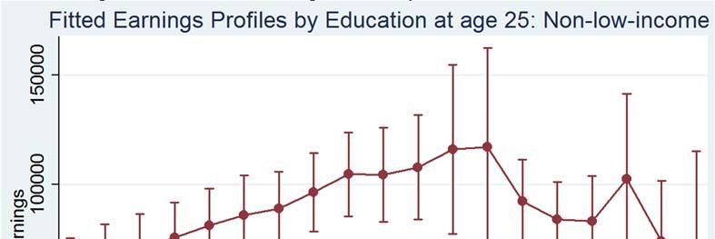
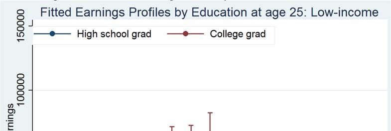
        We begin by presenting graphical career earnings profiles in Figures 1A and 1B, which

respectively show trajectories of mean earnings by education for individuals who grew up in low-income

families and for those who did not. Because the PSID switches to biennial surveying in 1997, we report

earnings by two-year age bins for consistency.

        In both graphs, college graduates earn considerably more than high school graduates throughout

the career, but this is not surprising. More interesting is the difference in slopes and levels of the profiles.

For high school graduates, the earnings slopes are quite similar across income backgrounds, with roughly

                                                       11

$700 increases every two years of age, although those from higher-income backgrounds earn about

$10,000 more at each age up to about age 50.13 In contrast, both slopes and levels diverge considerably

for college graduates. From the mid-20s through the mid-40s, low-income college graduates on average

increase their earnings by about $2,300 every two years, while higher-income college graduates have

average increases more than twice as large, at roughly $5,200 every two years. Furthermore, while

earnings appear to peak in the mid-40s for the former group, they continue to rise until age 50 for the

latter group. Together, these factors imply that the average college graduate who grew up in a low-income

family earns about as much at the peak of the career as the average college graduate from a higher-income

family whose career is just beginning.

        While these graphs are useful in illustrating when over the life cycle earnings differences occur,

we construct a summary measure of career earnings by taking the present discounted value of the profiles,

between ages 25 and 62, assuming a 3 percent discount rate and a base period of age 18. These values are

presented in Table 2. For individuals from low-income families who obtain only a high school diploma,

present discounted earnings are approximately $475,000, while for those who receive at least a bachelor’s

degree, this figure is about $810,000, a difference of $335,000 and a 70.6 percent increase. For

individuals from higher-income families, high school graduates earn about $661,000 over the career, or

about 39 percent more than individuals with the same level of education from poorer families. However,

average career earnings for bachelor’s graduates from the more well-to-do families reach $1.56 million.

Not only is this amount nearly two times what low-income bachelor’s graduates earn, it is 136 percent

more than what higher-income-background high school graduates earn.

        Put differently, the observed career earnings premium to (at least) a bachelor’s degree, relative to

a high school diploma, is nearly twice as large proportionally for individuals from non-low-income

families as it is for individuals from low-income families, 136 percent to 71 percent. This proportional

        13
          In proportional terms, the slope for low-income high school graduates is slightly larger, 2.7
percent compared to 2.0 percent, but not statistically significantly so.
                                                    12

difference is statistically significant at the 5 percent level and is quite large in practical terms. If low-

income-background college graduates received the same proportional boost to career earnings as their

peers from more fortunate backgrounds, their present discounted career earnings would be $1.12 million,

or $312,000 (38.5 percent) more than what they are observed to earn. If low-income-background college

graduates received the same dollar return to college graduation as their peers from higher-income

backgrounds, their present discounted career earnings would be $1.38 million, or $565,000 (69.9 percent)

more than their observed earnings. At an extreme, if a bachelor’s degree completely eliminated any

disadvantages associated with a low-income family background, and low-income-background college

graduates earned the same $1.56 million as their peers from higher-income backgrounds, this $1.56

million would represent a boost of $752,000 (92.9 percent) from their $810,000 in actual career earnings.

        To be clear, we are not claiming that coming from a low-income background causally reduces the

return to a bachelor’s degree. Rather, we find the magnitude of the observed correlational difference in

the premium striking, in part because the selection issues and literature described earlier suggest returns

should be (weakly) higher for those with a low propensity to complete college, and in part because such

large proportional differences are not observed across race or sex.14

        Of course, a myriad of factors could explain the relatively low earnings premium to college for

individuals from low-income backgrounds, including measurement issues inherent in the data as well as

more substantive issues. In the following subsections, we explore a number of features of these estimates

in an attempt to understand these estimates more fully.

        14
           Using the PSID data and the same approach, the observed proportional increase in present
discounted career earnings from a bachelor’s degree, relative to a high school diploma, is 137 percent for
(all) whites, 162 percent for blacks, 173 percent for men, and 119 percent for women. Similar findings are
obtained when one examines the cross-sectional (synthetic cohort) returns to education and how they vary
with age using data sets such as the Current Population Survey or the American Community Survey
(Bartik, Hershbein, and Lachowska 2016).
                                                       13

Decomposing Baseline Differences in Returns: College Versus High School Earnings

        How much of this large difference in relative percentage returns across family income

backgrounds is due to differences in college earnings versus differences in high school earnings? To do

such decomposition, it is convenient to reexpress the differences in the observed premium to a college

education in logarithmic differences, as shown in the top part of Table 3. For individuals who grew up in

a higher-income family background (greater than 185 percent of the poverty line), the 136.3 percent

career college earnings premium from Table 2 corresponds to a logarithmic value in Table 3 of 86 log

points (i.e., ln(2.363) × 100 = 86.0). For those who grew up in a lower-income family background (less

than 185 percent of the poverty line), the 70.6 percent college premium corresponds to 53.4 log points.

The log difference is thus 32.6 points in Table 3, which corresponds to the 65.7 percentage point

difference in Table 2.

        The advantage of this logarithmic formulation is that the difference across income groups in the

college earnings premium exactly equals the differences in the income background premium across

education groups. That is, Table 3 shows that, among those with a high school diploma only, the higher-

income background group actually earns about 33 log points more over the career than the lower-income

background group. But this difference across groups is roughly doubled, at 66 log points, for those who

earn a bachelor’s degree.

        As this discussion suggests, the differential return to a bachelor’s degree across income groups is

driven both by income background differences in the earnings of high school graduates and those in

college graduates (as well as selection into each education group). While both are empirically important,

the greater dispersion in the earnings of college graduates—which has been growing over time (Autor,

Katz, and Kearney 2006)—plays the larger role, and is a topic to which we return.

Further Exploring Differentials by Age

        Before considering variants to the baseline specification, we further explore earnings differentials

by age, beyond the picture provided by Figure 1. To do so, Table 4 considers the difference in predicted
                                                    14

earnings (logged) across the two income background groups, for each educational attainment category, by

two-year age bins. This formulation allows us to highlight how the differential education return varies

over the career.

        As shown in Table 4, log differences across income groups in earnings are quite similar at

younger ages for the two education groups, roughly around 30–40 points. But as individuals age, the log

differences between income background rapidly increase for the college-graduate group, through about

age 50, while remaining static for the high school graduate group. More specifically, log differences for

the former group reach 50 points during an individual’s 30s, and then rise to around 100 points as one

approaches age 50. In contrast, log differences in earnings for high school graduates generally stay

between 30 and 40 points into one’s 50s, although the estimates bounce around a bit at older ages.

        Thus, individuals from higher-income backgrounds earn greater proportional career returns from

completing college due to relative earnings increases that begin in the early 30s, accelerate rapidly until

about age 50, and then are maintained until the effective end of our sample, at ages in the early 60s.

However, it is worth noting that at the oldest of these ages the standard errors of our estimates increase

due to fewer earnings observations.15

Sensitivity to the Sample and to Weighting

        Our baseline estimates use the combination of the Survey Research Center (cross-sectional or

SRC) sample with the Survey of Economic Opportunity (low-income or SEO) sample of the PSID, with

the estimates weighted using PSID-provided weights. As explained above, we include the SEO sample

because we want more individuals with a low-income background in our estimation sample, precisely the

purpose of the SEO sample component.

        15
          The drop in predicted earnings for college graduates from low-income backgrounds (relative to
both high school graduates from the same background and to college graduates from more affluent
backgrounds; see Figure 1) also plays a role, albeit a smaller one due to the high discounting at these
ages.
                                                     15

We use weighting because the SEO oversamples lower-income persons, particularly in the South,

and weighting is necessary for sample statistics to approximate population statistics. However, while the

weights correct for representation by income background, they may not do so by education within income

background, which could threaten the representativeness of our estimates of differential educational

returns (Solon, Haider, and Wooldridge 2015).16

        To test the sensitivity of our results to such sample and weighting assumptions, Table 5 considers

alternative sampling choices using the PSID. We first consider two options: using only the nationally

representative SRC sample with sample weights, and using the SRC sample but without weights. It is

reassuring that the nationally representative SRC sample results are very similar to the weighted SRC-

SEO results. If anything, the differences in the returns to education across income background groups are

somewhat greater in the SRC sample, weighted or unweighted. For example, in the SRC weighted

sample, the log return to a college degree is 41 points for individuals from a low-income family

background, compared to 85 points for those individuals from a higher-income family background, a

difference of 44 log points. The baseline SRC-SEO weighted estimates show a difference of 33 log

points. Even without weighting, the SRC-only sample shows a difference of 37 log points. However,

because the SRC sample has fewer individuals in it with a low-income background, restricting estimation

to the SRC sample tends to increase standard errors somewhat, although not enough to change statistical

significance appreciably.

        On the other hand, when we use the unweighted SRC-SEO sample, the rate of return to education

for the low-income background group tends to increase, and the difference between the two groups in the

percentage return to a college education (using either absolute percentages or log differences) decreases

and is no longer statistically significant. A possible explanation of this phenomenon is provided by later

results in this paper, which suggests that returns to college education tend to be higher for individuals

with extremely low-income backgrounds. We suspect that the SEO oversample of such individuals tends

        16
             Brown (1996) discusses some of the sampling issues of the SEO oversample in the PSID.
                                                     16

to increase the rate of return to education. Weighting corrects for this phenomenon by making the low-

income-background group (less than 185 percent of poverty) more representative of the population from

this income background and less disproportionately from below the poverty line.

        The last row of Table 5 emphasizes that in all cases, even when the percentage returns to

education are no longer significantly higher for the higher-income group, the absolute dollar value of the

returns to college is still significantly higher for the latter group. For example, even in the SRC-SEO

unweighted sample, the career dollar return to a college education is $414,000 greater for individuals

from a higher-income background than it is for individuals from a low-income background. Both the

proportional and absolute return to college for the two income background groups may be of interest for

policy purposes.

Other Sample Restrictions

        Table 6 considers other restrictions in the estimation sample. First, rather than starting earnings at

age 25, we estimate conditional earnings starting at age 20. (The education groups are still classified by

education attainment as of age 25). This change adds career earnings for all education and income

background groups, but proportionally more for the high school graduate group, who spend more of this

age period working. While this reduces the career return to a college education, as expected, it does not

drop much differentially by family income background. Relative to the baseline case of a differential

across income groups of 32.6 log points, including earnings from age 20 reduces the differential only to

30.6 log points.17

        In the next column of Table 6, we exclude all observations with zero earnings, essentially

comparing earnings profiles of workers instead of all individuals. If education differentially affects the

likelihood of employment based on family income background, restricting the sample to observations

        17
           Note that the tendency of higher-income individuals to complete their degrees faster (and thus
have additional earnings between age 20 and 25 as college graduates) would tend to increase the log
differential. That it falls slightly suggests that relative earnings of high school graduates across income
groups play a role at these ages.
                                                     17

with positive earnings should shed light on the magnitude of this mechanism in driving the differential.

Perhaps unsurprisingly, this restriction slightly reduces the observed college premium for the low-

income-background group, as earnings increase proportionately more for high school graduates. For

individuals from a higher-income background, the proportional college premium also falls, but by

somewhat less. Therefore, this restriction actually increases the relative college premium for the higher-

income group, from about 33 log points at baseline to 42 points in the positive-earnings-only sample.18

        Finally, we consider dropping from the sample anyone who ever obtains a postcollege degree.

This restriction does make a major change to the earnings differential across income groups. In particular,

it significantly reduces expected lifetime earnings for the higher-income background group with a college

degree, from $1.56 million in the baseline sample to $1.23 million when those who obtain graduate

degrees are excluded. As a result, the estimated percentage rate of return to college falls substantially for

the higher-income background group, from 86 log points at baseline to 63 log points. This 63-point return

to college is not substantively or significantly different from the estimated 62 log point return to college

for the low-income background group, whose college premium actually rises slightly.19 The dollar return

to a college education for the higher-income background group still exceeds the dollar return for the low-

income background group, but by much less—the differential is only $205,000, relative to $566,000 at

baseline.

        The results from restricting the sample to those who never earn a graduate degree certainly

suggests that the college return differential by income background is a story more about advanced degrees

than bachelor’s degrees, per se. However, in the human capital investment framework, the additional

return that a graduate degree may bring is part of the option value to a bachelor’s degree. Under such a

        18
           This is consistent with larger differences in the likelihood of employment with greater
education among the low-income group, but the magnitude is relatively modest.
        19
           At age 25, 17.4 percent of bachelor’s graduates from the higher-income background group have
a graduate degree, while a similar 16.3 percent of graduates from the low-income group do. However,
these shares diverge with age. By age 30, they are 25.6 and 18.6 percent, respectively, and at the
maximum observed ages they are 36.5 and 27.8 percent.
                                                     18

conceptual framework, if individuals who grew up in a more economically advantaged family are more

likely to earn a graduate degree, conditional on earning a bachelor’s degree, then the advanced degree is a

possible mechanism for their proportionally greater return to earning (at least) a bachelor’s degree, and

one that has important implications for policies that promote undergraduate (but not necessarily

postgraduate) access and success. Moreover, compositional differences in who obtains a graduate degree

(and in what field) may also play a role, something to which we return below.

More Flexible Income Background Groups

         Although there is some reason to particularly focus on the free and reduced-price lunch cutoff, as

mentioned above, we want to explore more flexible specifications for how family income background

might affect the return to education. In Table 7, we consider as an alternative dividing individuals into

four groups by family income background: greater than 400 percent of the poverty line, 200–400 percent

of the poverty line, 100–200 percent of the poverty line, and below the poverty line. In examining the

return to a college degree, we compare each of the three lower-income groups to the highest-income

group.

         We find that the variation in the percentage return to a college degree follows a somewhat U-

shaped pattern with family income background. The biggest contrast in college premium is between the

highest-income-background group and the one with family income between 1 and 2 times the poverty

line. The highest-income group has a log return to a college degree of about 83 points, which is 44 points

higher than the 39-point return for the “near-poor” income group. The second-highest-income group

(200–400 percent of poverty) has a premium that is in between, at around 63 log points. But for

individuals who grow up below the poverty line, the observed college premium is remarkably high:

roughly 103 log points higher (but not statistically significantly so) than the 83 points of the highest-

income-background group. Additionally, the absolute dollar return for college graduates who grew up in

                                                      19

poverty is larger for all but the highest-income group, a pattern largely driven by the very low earnings of

individuals with only a high school diploma from the poorest group.20

        A comparison of the poverty-income group with the near-poor group is instructive. In log terms,

college graduates from the first group have earnings about 31 points greater than those from the second

group; among high school graduates, on the other hand, earnings are 32 log points less. Therefore, about

half of the 63.5 log point difference between these two groups in the return to college is due to the

difference in college earnings, and half is due to the difference in high school earnings.

        One interpretation of the relatively high earnings for college graduates from the poverty group is

selection: members of this group who earn a bachelor’s degree may have particularly high (unobserved)

skills, which are likely needed to overcome the greater barriers this group faces in getting a college

degree. On the flip side, the lower high school earnings of this group suggest its members face

particularly dire job prospects with limited education, perhaps because they lack the social capital (job

contacts or reputation) needed to get good jobs without a higher degree (Putnam 2015).

Looking Beyond Conditional Means to Other Moments of the Earnings Distribution

        Thus far we have looked only at the conditional means of earnings for different groups. In Table

8, we investigate other moments of the earnings distribution, which turns out to be important in

understanding the differential college premium by family income background.

        20
           Of the individuals who grew up in poverty in the sample, 15.8 percent earned a bachelor’s
degree by age 25. In ascending order for the remaining income groups, these shares are 18.5 percent, 36.7
percent, and 66.0 percent. Among those with bachelor’s degrees by age 25, the shares that ever obtain a
graduate degree are 22.2, 30.8, 31.0, and 40.8 percent. Thus, it is interesting that those who grow up in
poverty have the highest college premium despite the smallest share earning a graduate degree. That the
college premium is proportionally lower for those below the 185 percent of poverty threshold, but not at
the 100 percent threshold, is a result of the relatively greater number of college graduates (and relatively
fewer high school graduates) who grew up with family incomes between 100 and 185 percent of the
poverty line.
                                                     20

First, we examine the impact of outliers by simply eliminating all observations that are in the top

1 percent of the sample earnings distribution in each survey wave.21 Doing so greatly reduces the

differential in the observed college earnings premium between the two income background groups, and

the remaining difference is no longer statistically significant. The predominant effect of dropping the top

1 percent of earnings observations mainly is to reduce mean expected earnings for the higher-income

background group with a college degree, from $1.6 million in lifetime earnings to $1.2 million. This

lowers the log return to college education for the higher-income background group from 86 points to 60

points, which is no longer significantly greater than the (almost unchanged) 53-point return for the low-

income group. (Absolute dollar returns are still significantly greater, at $204,000, but this is less than half

the difference when the full earnings distribution is included.) These results suggest, in line with the

graduate degree results in Table 6, that the baseline numbers are driven in no small part by some college

graduates from the higher-income background group who obtain very high earnings in some years. We do

not believe that this apparent differential access to the far-right tail of the earnings distribution—even for

college graduates—for those from different income backgrounds obviates our baseline results. On the

contrary, a host of work by Piketty and Saez and many others documents the fastest relative income

growth at the top of the earnings distribution.22 If individuals from low-income backgrounds are less

likely to have access to this part of the earnings distribution—even with high levels of education—there

may be considerable consequences for both earnings inequality and intergenerational mobility.

        To further illustrate the importance of the tails of the earnings distribution, we consider earnings

at different percentiles of that distribution, specifically earnings at the 25th percentile, the median, the

75th percentile, and the 90th percentile. These are shown in the remaining columns of Table 8. At the

25th percentile, the log return to college is actually much higher (175 points) for individuals from low-

        21
            Earnings are not top-coded in the PSID. The 99th percentile of sample earnings (in $2014)
varies from approximately $75,000 in the mid-1970s, when the oldest sample respondent is in her mid-
20s, to about $400,000 before the Great Recession, when the oldest sample respondent is in her late 50s.
         22
            Autor, Katz, and Kearney (2008) provide a review.
                                                      21

income backgrounds than it is for those from high-family-income backgrounds (87 points), and even the

absolute dollar return is slightly higher. This apparent reversal from baseline occurs for two reasons. First,

at the 25th percentile of the earnings distribution, earnings for high school graduates from a low-income

family essentially collapse, decreasing from $475,000 at the mean to just $83,000 at the 25th percentile.

Earnings for high school graduates from higher-income families fall as well, but not by as much, from

$661,000 to $226,000. Apparently, the lower tail of earnings for low-income-background high school

graduates is quite low indeed. Second, at the 25th percentile, earnings for college graduates are not that

different for individuals from the different income backgrounds; both are approximately $500,000. In

conjunction with the results from excluding the extreme right tail, these patterns suggest not only a much

larger variance in earnings for college graduates coming from a higher-income background than for

college graduates from poorer families, but that the lower tail of earnings is fairly similar for both groups.

Put differently, a higher-income background—conditional on having a bachelor’s degree—stretches the

right tail of the earnings distribution.

        Switching to the median, we find that the relative (log) return to college is slightly (not

statistically significantly) higher for the low-income group, and that the absolute dollar returns are similar.

Thus, the median or typical college graduate enjoys an earnings return that does not vary much with her

family income-background, in contrast with the “average” college graduate. This again emphasizes the

importance of the tails of the earnings distribution.

        The higher percentage return to college for the higher-income-background group begins to re-

emerge as we move to the 75th and 90th percentiles. However, these percentage returns are only weakly

significantly higher for the higher-income-background group, in part because the standard errors for the

low-income-background group tend to increase, due to diminished density, higher up in the earnings

distribution. The dollar returns to a college degree, however, are both substantively and statistically much

greater for the higher income group at the 75th and 90th percentiles. For example, at the 90th percentile, a

college degree increases lifetime earnings for the higher-income-background group by almost $1.4

                                                        22

million, compared with just under $500,000 for the low-income-background group. This difference of

almost $900,000 is clearly statistically (and economically) significant.

        Overall, a striking pattern is that at the various percentiles, the dollar return to a college degree

remains fairly flat, between roughly $400,000 and $500,000, for the low-income background group. In

contrast, the dollar return to a college degree for the higher-income background group dramatically

escalates as when moving from lower to higher percentiles, increasing from a little over $300,000 to

almost $1.4 million between the 25th percentile and 90th percentiles. Once again, the right tail of the

earnings distribution for college graduates who come from low-income families is considerably shorter

than it is for their peers from more-affluent families.

        This quantile analysis is illustrative, but the importance of location in the earnings distribution in

contributing toward the family background college earnings gap can perhaps most clearly be seen by

looking at the entire earnings distribution. We present the summary measure of the ratio difference in

Figure 2. In the figure, the x-axis represents the percentile of the cumulative career earnings distribution,

and the y-axis represents the difference in the ratio at a given cumulative earnings percentile.23 Since the

bottom quarter of the earnings distributions consists of zeroes or very small values, which make ratios

unstable or infeasible to calculate, we focus on the top three quartiles of the distribution. From the 25th

percentile to about the 45th percentile, the calculated ratio difference is negative, implying that the

observed proportional college earnings premium is actually higher for individuals from low-income

families than it is for those from higher-income families. However, as the bootstrapped confidence

intervals show, a null of no difference in the ratios cannot be rejected. The ratio difference is actually

weakly positive at the median, but again a zero difference lies within the confidence interval, consistent

        23
           To calculate these distributions for each family-income–education group, we create 5,000
bootstrap replication draws of individuals, with replacement, from the analytic sample. For each group in
each replicate draw, we estimate the empirical cumulative distribution function at each age, and then sum
across ages for each centile of the cumulative distribution function. This yields 5,000 replicates of
cumulative career earnings at each centile for each group. We calculate the ratio difference for each
centile of each replicate and then take the median of the ratios across replicates.
                                                      23