DISCUSSION PAPER SERIES - DP15826 Who Bears the Burden of Local Taxes? Marius Brülhart, Jayson Danton, Raphael Parchet

DISCUSSION PAPER SERIES

 DP15826

Who Bears the Burden of Local Taxes?

 Marius Brülhart, Jayson Danton, Raphael Parchet
 and Jörg Schläpfer

 PUBLIC ECONOMICS

ISSN 0265-8003

 Who Bears the Burden of Local Taxes?
 Marius Brülhart, Jayson Danton, Raphael Parchet and Jörg Schläpfer

 Discussion Paper DP15826
 Published 18 February 2021
 Submitted 17 February 2021

 Centre for Economic Policy Research
 33 Great Sutton Street, London EC1V 0DX, UK
 Tel: +44 (0)20 7183 8801
 www.cepr.org

This Discussion Paper is issued under the auspices of the Centre’s research programmes:

 Public Economics

Any opinions expressed here are those of the author(s) and not those of the Centre for Economic
Policy Research. Research disseminated by CEPR may include views on policy, but the Centre
itself takes no institutional policy positions.

The Centre for Economic Policy Research was established in 1983 as an educational charity, to
promote independent analysis and public discussion of open economies and the relations among
them. It is pluralist and non-partisan, bringing economic research to bear on the analysis of
medium- and long-run policy questions.

These Discussion Papers often represent preliminary or incomplete work, circulated to encourage
discussion and comment. Citation and use of such a paper should take account of its provisional
character.

Copyright: Marius Brülhart, Jayson Danton, Raphael Parchet and Jörg Schläpfer

Who Bears the Burden of Local Taxes?

 Abstract
 We study the incidence of local taxes on the welfare of heterogeneous residents. A structural
 model of imperfectly mobile households who differ in terms of income and family status allows us
 to back out preferences for local public goods and mobility parameters that vary by family status.
 We calibrate the model with plausibly causal tax-base and housing-price elasticity estimates.
 Based on municipality-level data for Switzerland, we find that households with children have
 stronger preferences for locally provided public services and are less mobile than households
 without children. This in turn implies that the burden of local taxes is mainly borne – linearity of
 taxes and capitalization into lower housing notwithstanding – by above-median income households
 without children.

 JEL Classification: H24, H71, R21, R31

 Keywords: Tax Incidence, Local taxation, public-good preferences, household mobility,
 heterogeneous households, housing prices

 Marius Brülhart - marius.brulhart@unil.ch
 University of Lausanne and CEPR

 Jayson Danton - jaysonmarc.danton@snb.ch
 Swiss National Bank

 Raphael Parchet - raphael.parchet@usi.ch
 Università della Svizzera italiana

 Jörg Schläpfer - joerg.schlaepfer@wuestpartner.com
 Wüest Partner AG, Zurich

 Acknowledgements
 We thank Jan Brueckner, Pierre-Philippe Combes, Jonathan Dingel, Jessie Handbury, Christian Hilber, Patrick Kline, Jean-Paul
 Renne, Frédéric Robert-Nicoud, Mark Schelker, Kurt Schmidheiny, Sebastian Siegloch, David Wildasin, and seminar and
 conference participants at the 2021 Econometric Society Winter Meetings, the Universities of Barcelona (IEB), Basel, Bergamo
 (Winter Symposium), Bern, Columbia (UEA), Duisburg, Fribourg, Geneva, Glasgow (IIPF), Helsinki GSE, LSE (SERC), Lyon
 (GATE), Mannheim (ZEW), Milan, Naples Federico II, Rome (Banca d’Italia), Siegen, Turin (SIEP), Venice (CESifo Summer
 Institute), Vienna, and Zurich for helpful comments. Funding from the Swiss National Science Foundation (grants 147668, 159348,
 182380 and 192546) is gratefully acknowledged. We are particularly indebted to the Swiss Federal Tax Administration, Wüest
 Partner, and to Laura Fontana-Casellini for granting us access to their data. The views, opinions, findings, and conclusions or
 recommendations expressed in this paper are strictly those of the authors. They do not necessarily reflect the views of the Swiss
 National Bank or Wüest Partner. The SNB and Wüest Partner take no responsibility for any errors or omissions in, or for the
 correctness of, the information contained in this paper.

Powered by TCPDF (www.tcpdf.org)

Who Bears the Burden of Local Taxes?*

 Marius Brülhart† Jayson Danton‡
 University of Lausanne Swiss National Bank

 Raphaël Parchet§ Jörg Schläpfer¶
 Università della Svizzera italiana Wüest Partner

 February 18, 2021

 Abstract

 We study the incidence of local taxes on the welfare of heterogeneous residents. A
 structural model of imperfectly mobile households who differ in terms of income and
 family status allows us to back out preferences for local public goods and mobility pa-
 rameters that vary by family status. We calibrate the model with plausibly causal tax-base
 and housing-price elasticity estimates. Based on municipality-level data for Switzerland,
 we find that households with children have stronger preferences for locally provided pub-
 lic services and are less mobile than households without children. This in turn implies
 that the burden of local taxes is mainly borne – linearity of taxes and capitalization into
 lower housing notwithstanding – by above-median income households without children.

 JEL Classification: H24, H71, R21, R31
 Keywords: tax incidence, local taxation, public-good preferences, household mobility, housing
 prices

 * We thank Jan Brueckner, Pierre-Philippe Combes, Jonathan Dingel, Jessie Handbury, Christian Hilber, Patrick
Kline, Jean-Paul Renne, Frédéric Robert-Nicoud, Mark Schelker, Kurt Schmidheiny, Sebastian Siegloch, David
Wildasin, and seminar and conference participants at the 2021 Econometric Society Winter Meetings, the Uni-
versities of Barcelona (IEB), Basel, Bergamo (Winter Symposium), Bern, Columbia (UEA), Duisburg, Fribourg,
Geneva, Glasgow (IIPF), Helsinki GSE, LSE (SERC), Lyon (GATE), Mannheim (ZEW), Milan, Naples Federico II,
Rome (Banca d’Italia), Siegen, Turin (SIEP), Venice (CESifo Summer Institute), Vienna, and Zurich for helpful
comments. Funding from the Swiss National Science Foundation (grants 147668, 159348, 182380 and 192546) is
gratefully acknowledged. We are particularly indebted to the Swiss Federal Tax Administration, Wüest Partner,
and to Laura Fontana-Casellini for granting us access to their data. The views, opinions, findings, and conclusions
or recommendations expressed in this paper are strictly those of the authors. They do not necessarily reflect the
views of the Swiss National Bank or Wüest Partner. The SNB and Wüest Partner take no responsibility for any
errors or omissions in, or for the correctness of, the information contained in this paper.
 † Department of Economics, Faculty of Business and Economics (HEC Lausanne), University of Lausanne, 1015

Lausanne, Switzerland; and CEPR, London. (Marius.Brulhart@unil.ch).
 ‡ Swiss National Bank, Financial Stability, 3001 Bern, Switzerland. (JaysonMarc.Danton@snb.ch).
 § Institute of Economics, Faculty of Economics, Università della Svizzera italiana (USI), 6900 Lugano, Switzer-

land. (raphael.parchet@usi.ch).
 ¶ Wüest Partner AG, Bleicherweg 5, 8001 Zurich, Switzerland (joerg.schlaepfer@wuestpartner.com).

Introduction
The distributional effects of taxation are among the most studied topics in public finance. Ex-
isting research has mainly focused on taxes at the national level. In this paper, we study the
distributional effects of local taxation, which accounts for important shares of public revenue
in many countries. For example, taxes raised by cities, counties, school districts or munic-
ipalities represent 16% of total tax revenues in Switzerland, 15% in the United States, 10%
in Canada, 9% in Spain and 8% in Germany.1 Most local taxes are levied on the income or
property of residents and are used to finance locally provided public goods, notably school-
ing.2 This in turn affects resident households differently depending on their family status
and income.
 We consider two distinctive aspects of local taxes: changes in taxation are typically linear
or only weakly progressive, and tax bases are mobile – but not perfectly so. In addition,
we allow preferences for housing and locally funded public goods to be non-homothetic.
In this setting, distributional effects arise because capitalization of tax rates into housing
prices affects different households differently, and because households have unequal needs
for locally funded public goods.3
 We estimate a structural model using new panel data for Swiss municipalities, and we
find substantial heterogeneity in the incidence of municipal taxation across family types. For
childless households, the welfare effect of a one-percent increase in the local tax rate ranges
from slightly positive (+0.05%) for below-median income households to strongly negative
for top-quartile income households (−0.28%). When considering families with children, the
incidence of local taxes is more positive across all income classes, ranging from +0.24% for
below-median households to −0.05% for top-quartile income households. Underlying these
welfare effects are two structural parameters that we estimate. On the one hand, we find that
preferences for locally provided public goods are around 2.5 times stronger for households
with children compared to those without children. On the other hand, estimated household
mobility appears to be an order of magnitude higher for households without children than
for households with children. While our estimates are identified by variations in local income
taxes and in rental prices, our analytical framework as well as our qualitative findings apply
also to other residence-based local taxes (e.g. property taxes) and to owner-residents.
 The central mechanism we study can be illustrated as follows. Consider a linear increase
in a locality’s tax rate, associated with a corresponding increase in local expenditure e.g. on
elementary schools and daycare facilities. Families with children – who may attach more
weight to local public expenditure than childless households – will be attracted (or repelled
 1 Data from the OECD Fiscal Decentralization Database for the period 2000-2017. This list includes only coun-
tries with a three-tier jurisdictional architecture. In some two-tier federations, the local share is even higher (e.g.
34% in Sweden, 28% in Denmark).
 2 In the United States, some 47% of local own-source general revenue are raised through property taxation,

and some 3% are raised through income taxation. Primary and secondary education accounts for 40% of U.S.
local government spending (Annual Survey of State and Local Government Finances, Tax Policy Center, 2020). In
Switzerland, income and property taxation account for 43% and 5% of local governments’ own revenue, respec-
tively, and 27% of local expenditure are allocated to schooling (see Section 2.1).
 3 In contrast, at the national level, the tax system most evidently redistributes through the progressivity of rate

schedules and because of differential avoidance opportunities.

 1

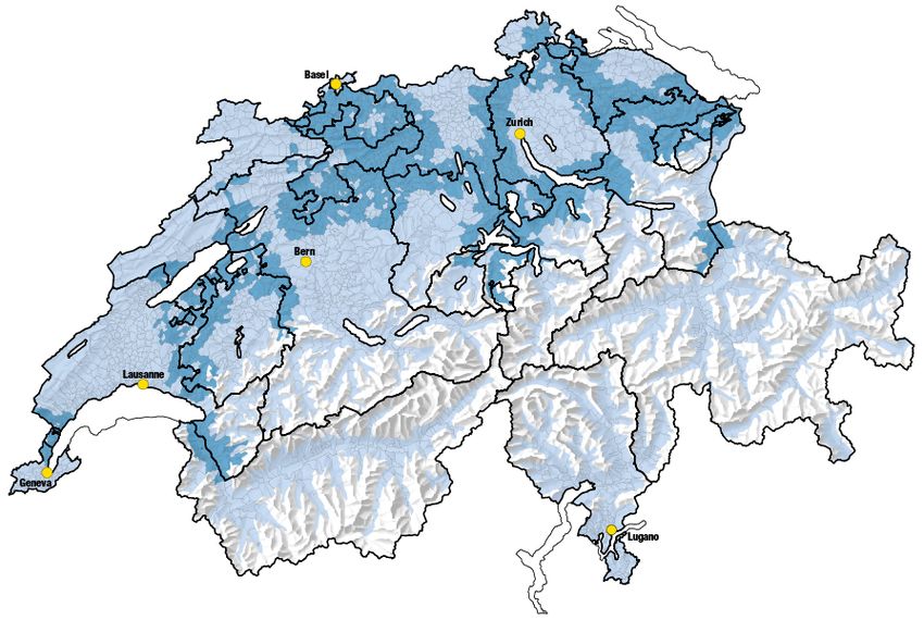
Figure 1: Revelealed locational preferences: family status, income and local tax rates

 without children with children
 80

 80
 70

 70
 Share of municipal tax base (%)

 Share of municipal tax base (%)
 60

 60
 slope = -0.97
 50

 50
 40

 40
 slope = 0.35
 30

 30
 20

 20
 10

 10
 0

 0
 4 6 8 10 12 14 16 18 20 22 4 6 8 10 12 14 16 18 20 22
 Tax rate (in %) Tax rate (in %)

 (a) (b)

Notes: The figure presents the share of the municipal tax base accruing to working-age households without children (left panel)
and with children (right panel). Within a panel, each circle represents a municipality. Municipalities are ranked according to the
average tax rate on top 10%-income households. Circle size and color intensity varies with average income by family type and
municipality. Four circle sizes are considered, denoting average incomes below 50,000 CHF, between 50,000 and 75,000 CHF,
between 75,000 and 100,000 CHF, and above 100,000 CHF, respectively. Lines are OLS linear fits (robust standard error in both
cases: 0.06). Data are for 2004.

less) by the tax increase. As a result, the demographic composition of the jurisdiction shifts
towards families with children. Suppose also that the tax increase leads to lower equilibrium
housing demand and thus housing prices.4 If lower-income households with children spend
a higher share of their budget on housing than higher-income childless households, then cap-
italization will reduce lower-income households’ direct loss from the higher tax rate relatively
more, and attract them (even more) into the higher-tax jurisdiction. Non-homothetic housing
demand can thus imply an asymmetric effect of a tax increase both according to income and
family status. As a result, even a linear change in taxation may not be distributionally neutral.
The ordering and even the sign of welfare effects on different household types will depend
on their relative mobility and preferences for locally provided public goods – parameters that
we estimate –, and on their relative housing needs – a parameter that we calibrate.
 Figure 1 provides some prima facie evidence of revealed preferences that systematically
differ according to family status and income. Using our data for Swiss municipalities, we
show the income share of working-age households without children (left panel) and with
children (right panel). Each circle represents a municipality, ranked horizontally by its average
tax rate. Circle size and color intensity reflects average household incomes in the given
municipality. Average incomes differ considerably across municipalities, ranging from 32,000
USD in the poorest sample municipality to 166,000 USD in the wealthiest municipality.5 The
graph shows that poorer households of both types account for a larger population share in
high-tax municipalities. Households with children sort disproportionately more into high-
tax municipalities while childless households sort more strongly into low-tax jurisdictions.
 4 The net effect of a tax increase on the population size of the jurisdiction depends on the relative preference

for the local public good by households with and without children.
 5 We use the 2014 exchange rate of 1.10 USD per 1 CHF. The stated range corresponds to the 1st and the 99th

percentile of the distribution of per-capita incomes across municipalities.

 2

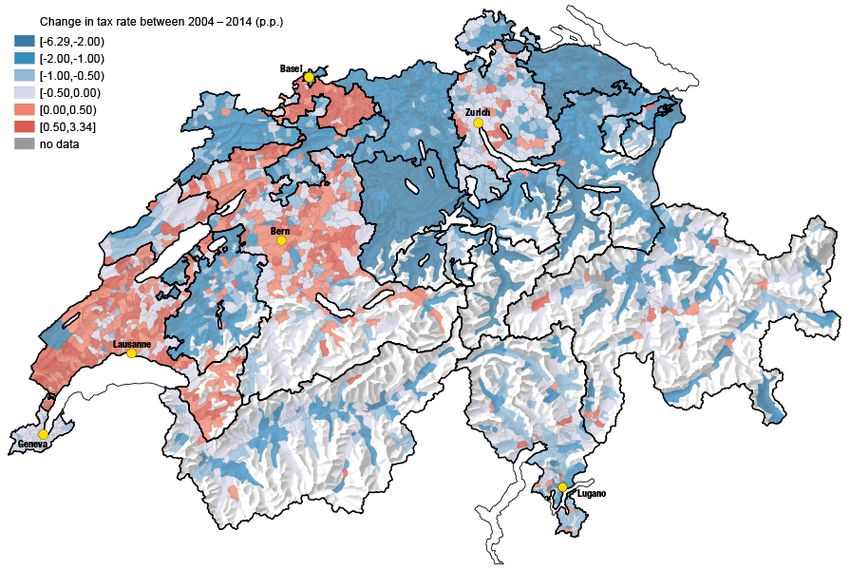
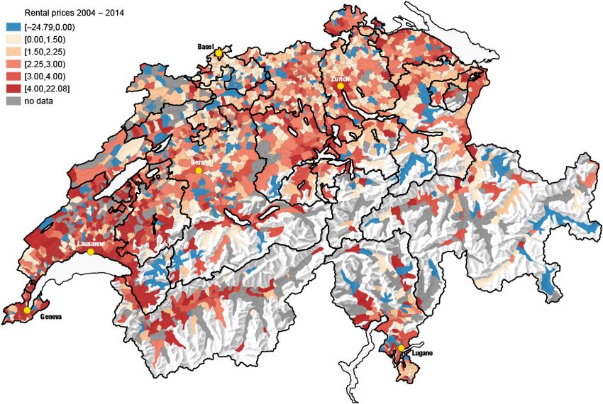
Poorer households and families with children thus appear to be deterred less by high local
taxes.
 The cross-sectional patterns illustrated by Figure 1 are purely correlational, and the di-
rection of causation could run from household composition to tax rates. For a causal anal-
ysis of the effect of changing tax rates, we first exploit intertemporal variation and estimate
reduced-form elasticity parameters based on changes in local tax rates and income-class-
specific taxpayer counts in the population of Swiss municipalities, as well as on 1.6 million
transaction-level rental price postings covering all of Switzerland over the 2004-2014 period.
Second, the Swiss institutional setting, featuring three jurisdictional layers, each with large
autonomy to tax and spend, allows us to instrument changes in local tax rates. This is a
unique advantage of our setting that permits us to estimate causal effects of changes in local
taxes. We follow Parchet (2019) and exploit cross-section and time variation in municipal tax
rates at state (‘canton’) borders, instrumented with neighboring state-level tax rates.
 We find the sensitivity to local taxes to differ markedly across household types: tax base
elasticities with respect to tax rates are positive for below-median income households (0.15
and 0.09 for households without and with children, respectively), strongly negative for top-
quartile income households without children (-1.11), and not significantly different from zero
for top-quartile households with children. The housing price elasticity with respect to local
income taxes is -0.30.
 In a next step, we use these reduced-form elasticity estimates to calibrate a model with
non-homothetic housing demand, household-type specific preferences for publicly provided
goods, and household-type specific mobility in order to estimate those unobservable model
parameters structurally. Residents are assumed to be imperfectly mobile and to rent hous-
ing from absentee landlords, with upward-sloping local housing supply. Households choose
where to reside among jurisdictions that offer different public expenditure levels, financed
by a proportional income tax on residents. We allow residents’ valuation of the locally pro-
vided public good to vary by family status, without imposing any prior restriction on this
relationship. Household types are defined in terms of income, to allow for preference non-
homotheticity, and of the presence or absence of dependent children, to account for different
needs for publicly provided goods and for different mobility. In an extension, we in addi-
tion distinguish pension-age from working-age households. In this setting, the incidence of
changes in local tax rates on households depends on their their type-specific ‘bid-rent’ price,
i.e. their marginal willingness to trade off taxes and public spending against housing prices.
We use equilibrium conditions for location choices and for local housing markets to derive
theoretical reduced-form effects of a tax increase on the number of households per type and
on housing prices. The theoretical reduced-form elasticities are determined by three key
parameters: family-status-dependent preferences for the local public good, the price elastic-
ity of housing supply, and the family-status-dependent dispersion of idiosyncratic locational
preferences that captures residential mobility.
 One specificity of our approach is that we focus on changes in local taxes within a given
functional labor market or commuting area. We therefore treat wages as exogenous with
respect to location choices. This allows us to take account of residential mobility while as-

 3

suming a constant labor income. The assumption of locally exogenous wages has empirical
support: Löffler and Siegloch (2018) find no effect of local property taxes on local wages,
which is all the more remarkable considering that their German sample municipalities are
on average almost 20 times larger than our Swiss sample municipalities. Martínez, Saez and
Siegenthaler (2021) find earnings responses to changed tax rates to be very small in Switzer-
land.6 Even though we analyze sorting and tax incidence at small spatial scale, however, we
consider a utility cost of moving. This contrasts with much of the literature on sub-national
public finance, following Tiebout (1956) and Oates (1969), where residential mobility is cost-
less. With perfect mobility, the incidence of local taxes is fully borne by landowners, the
immobile factor. In reality, moving costs exist even at the local level, and hence the welfare
of renter households will also be affected by changes in local taxation. We therefore assume
households to have idiosyncratic prior preferences over locations, and thus non-zero moving
costs, even within a given labor market. These moving costs are allowed to depend on family
status.
 Our study contributes to four main strands of the literature. First, we build on and con-
tribute to an active research program studying the incidence of subfederal taxation by taking
careful account of capitalization effects. In a seminal paper, Suárez Serrato and Zidar (2016)
use structural estimation to apportion the incidence of U.S. state corporate tax rates to work-
ers, landowners and firm owners. They estimate that some 40 percent of the gain from
state-level corporate tax cuts accrue to firm owners and 30-35 percent accrue to workers.7
Löffler and Siegloch (2018) focus on local property taxation in Germany and explicitly con-
sider locally provided public goods. They find that renter households bear one fifth of the
incidence of property taxes. Schönholzer and Zhang (2017), study municipal annexations in
the United States and similarly find most of the incidence of local public spending to accrue
to property owners. Importantly, they estimate substantial valuations by residents of locally
provided public goods.
 Our paper differs from this work along the following main dimensions. Most impor-
tantly, we estimate distributional effects by disaggregating residents by family status and
income (and, in an extension, age). To do so, we structurally estimate the relationship be-
tween revealed public-goods preferences and family status.8 Methodologically, we address a
key identification issue by instrumenting local tax rates. We moreover use housing demand
shifters to estimate the housing supply elasticity – an important parameter governing the
 6 This is of course not to deny that labor supply and wages are affected by subfederal income taxation at
larger spatial scales, such as that of U.S. states (see, e.g., Zidar, 2019). We also abstract from strategic interac-
tions among municipalities in their tax setting. Our thought experiment involves a shock to the tax rate of one
municipality without taking account of possible second-round effects through strategic responses by neighboring
municipalities.
 7 The share of corporate-tax incidence falling on workers has been found to be even higher in smaller jurisdic-

tions. Based on reduced-form empirical moments, Fuest, Peichl and Siegloch (2018) estimate that half of the gains
from cuts to municipal business tax rates in Germany accrue to workers. This effect is mainly driven by small,
single-plant (and thus immobile) firms.
 8 Suárez Serrato and Wingender (2016) study the incidence of federal government spending at the local level

and structurally estimate separate preference parameters for skilled and unskilled workers. Fajgelbaum, Morales,
Serrato and Zidar (2019) allow worker preferences for the public good to differ across U.S states. We also comple-
ment Eugster and Parchet (2019), who use the Swiss language border to show the effect of culture on preferred
tax levels, without, however, considering heterogeneity across household types.

 4

welfare effects of local policies (Kline and Moretti, 2014).
 Second, we contribute to a well developed empirical literature on the capitalization of
taxes in housing prices.9 Like us, Basten, Ehrlich and Lassmann (2017) draw on Swiss micro-
geographic data to estimate the capitalization of local taxes into housing prices. In line with
the empirical literature on the capitalization of local policies or amenities, they use a (bor-
der) regression discontinuity framework and assume that, locally, households are perfectly
mobile and housing demand is perfectly elastic.10 Reduced-form estimates of house price
responses then serve directly as a measure of willingness to pay (through housing prices),
but the incidence of the tax is assumed to be fully borne by the immobile factor. The perfect-
mobility assumption is implied also in the discrete choice framework developed by Bayer
et al. (2007), where housing and neighborhood characteristics are interacted with household
characteristics. We instead take a structural approach to estimate the elasticities that need to
be calibrated for an analysis of incidence on different types of imperfectly mobile households,
taking account not only of non-homothetic preferences for housing but also of heterogenous
preferences for local public goods and differential mobility across household types.
 Third, we complement the empirical literature on the mobility response of households to
tax changes.11 This literature is largely focused on top-income taxpayers and leaves mobility
responses of middle-income and lower-income households still to be explored. Tax-induced
mobility has previously been found to be significant in the case of Switzerland, probably due
to the combination of high degree of fiscal decentralization and a small spatial scale.12 We
link type-specific tax base elasticities to taxpayers’ marginal willingness to pay and study the
distributional effects of local tax changes.
 Fourth, our results shed light on the empirical relationship between local spending and
the demographic composition of local populations. A considerable prior literature exists on
this issue.13 In those papers, heterogeneous preferences are allowed, but no attempt is made
to back out deep type-specific preference parameters. We back out preference parameters
through structural estimation. In doing so, we show that mobility and preferences for locally
provided public goods differ substantially across family types.14
 The paper proceeds as follows.15 In Sections 1 and 2, we present a model of local labor
and housing markets and the data that will inform our empirical estimations. In Section 3
we estimate reduced-form elasticities of tax bases and housing prices with respect to local tax
 9 Seminal studies of the capitalization of property taxes include Epple and Zelenitz (1981) and Yinger (1982).

See Ross and Yinger (1999) and Hilber (2015) for comprehensive surveys.
 10 See, e.g., Black (1999); Reback (2005); Bayer, Ferreira and McMillan (2007); Fack and Grenet (2010); Cellini,

Ferreira and Rothstein (2010); Black and Machin (2011); Boustan (2013); Gibbons, Machin and Silva (2013).
 11 See, e.g., Kleven, Landais and Saez (2013); Moretti and Wilson (2017); Agrawal and Foremny (2019); Kleven,

Landais, Muñoz and Stantcheva (2020).
 12 See, e.g., Schmidheiny and Slotwinski (2018); Brülhart, Gruber, Krapf and Schmidheiny (2019); Martínez

(2017); Widmann (2019).
 13 See, e.g., Harris, Evans and Schwab (2001); Hilber and Mayer (2009); Aaberge, Bhuller, Langørgen and

Mogstad (2010); Figlio and Fletcher (2012); Bertocchi, Dimico, Lancia and Russo (2020); Aaberge, Eika, Langørgen
and Mogstad (2019).
 14 On residential income segregation by households with and without children, see, e.g., Epple, Romano and

Sieg (2012) and Owens (2016). For evidence on residential sorting by household type according to differences in
exogenous local amenities (rather than local public goods), see, e.g., Chen and Rosenthal (2008) and Albouy and
Faberman (2019).
 15 Appendix A.1 offers a schematic overview of the different building blocks of the paper.

 5

rates. Section 4 reports our baseline structural type-specific incidence estimates. In Section 5,
we present some extensions of the baseline estimations, and Section 6 concludes.

1 Model
In this Section, we develop a model of residential location choice, housing markets and local
public good provision. First, we assume a public sector that uses a proportional income tax to
provide a potentially rival publicly provided good, and we characterize location choices and
housing demand by households that differ by family status and income.16 Second, we model
housing supply in an absentee landlord setting. Third, we use the model to investigate the
effect of tax rate changes on housing prices, on the number of residents in different family
status-income class pairs (“household types”), and, most importantly, on the incidence of
local taxes across household types.

1.1 Housing demand
We assume a functional labor market that consists of J municipalities. This labor market
is populated by a unit continuum of I households that rent dwelling space from atomistic
absentee landlords and take housing prices as given. Households have identical preferences
for housing and public goods but are heterogeneous in their family status (with/without
children) and income.17 We assume Stone-Geary preferences with minimum levels of housing
and public good consumption that depend on family status, thus capturing different needs
for residential space and public services by families with and without children. We also
assume that households derive idiosyncratic utility from exogenously given local amenities.
 Specifically, each of the i ∈ I renter households belongs to a discrete family status f ∈ F
and income class m ∈ M. Within an income class, everybody’s income equals wm . House-
holds maximize the log Stone-Geary utility of residing in municipality j ∈ J by choosing
consumption levels of a freely tradable numeraire composite good zf mj and dwelling size
hf mj , at a rental price pj , subject to their after-tax income (1 − τj )wm .
 The indirect utility of household i with family status f and income wm , based on its choice
of location j, is
 h i
 Vif mj = κ + ln (1 − τj )wm − pj νhf − α ln(pj ) + δ ln(gj − νgf ) + ln(Aif j ) , (1)

where κ is a constant, α ∈ (0, 1) and δ are taste parameters for housing and the local public
good, and νhf ≥ 0 and νgf ≥ 0 are Stone-Geary parameters capturing the family type-specific
minimum amount of housing and public good required, respectively.18 The Stone-Geary
parameters play an important role. First, unlike e.g. a Cobb-Douglas function, they al-
low for a full range of housing demand elasticities with respect to the price of housing, i.e.
|η d,p | ∈ (0, +∞). Second, households with different family status and income have different
 16 For simplicity, we use the term “public goods” as equivalent to “publicly provided goods”. Our setting can
easily be extended (a) to other residence-based taxes such as a property tax, and (b) to homeowners as in, e.g.,
Epple and Romer (1991).
 17 When we take the model to the data, we shall in addition distinguish household types by age, that is, we

consider three family statuses: non-pensioners without children, non-pensioners with children, and pensioners.
 18 See Online Appendix W.1 for detailed derivations.

 6

expenditure shares on housing, such that the capitalization of higher tax rates into housing
prices will affect them differently.19 Third, νgf allows for the fact that households with chil-
dren have different needs in terms of goods such as schooling than childless households, and
might therefore benefit more from an increase in the public good.
 We furthermore assume a balanced budget for the public sector with τj ∑f ∑m wm Nf mj =
Njθ gj ,
 where θ ∈ [0, 1] indicates the degree of rivalness in the consumption of the public
good.20 The number of residents, Nf mj , is defined below. We also assume local amenities
Aif j to be fixed.21
 At this stage, it is useful to define the change in the housing price (‘bid-rent’ price change)
a household with family status f and income wm would require to be indifferent toward a
given change in the local tax rate:
 " ! ! #
 dpj τj τj δ gj νhf dgj τj
 =− − 1− ∗ , (2)
 dτj pj
 dVif mj =0
 (1 − τj )Sf mj α gj − νgf hf mj dτj gj

where Sf mj ≡ pj hf∗ mj /(1 − τj )wm represents the housing expenditure share and hf∗ mj is the
 dgj τj
household’s Marshallian demand for housing space. dτj gj is the elasticity of public good
provision with respect to the local tax rate. Using the balanced budget constraint, we have

 dgj τj dNf mj τj
 = 1 + ∑ ∑(γf mj − θsf mj ) , (3)
 gj dτj f m
 Nf mj dτj

where γf mj ≡ wm Nf mj / ∑f ∑m wm Nf mj represents household type {f , m}’s share of munic-
 dN mj τj
ipality j’s tax base, sf mj is the proportion of households of type {f , m}, and Nffmj dτj is the
elasticity of the number of residents belonging to household type {f , m} with respect to the
local tax rate.
 Expression (2) determines the household type {f , m}’s marginal willingness to pay rent
(MWPR) for a (small) tax rate change. It differs across household types {f , m} through the
family status-specific minimum consumption of housing and public goods. In particular, if
νhf = νgf = 0 then Sf mj = α and the MWPR becomes type-invariant.
 We incorporate imperfect residential mobility by modeling location-specific amenities
Aif j , consisting of a common location-specific component Aj and a location-specific idiosyn-
cratic preference component ξif j . The household’s objective is therefore to maximize
 h i
 max Vif mj = κ + ln (1 − τj )wm − pj νhf − α ln(pj ) + δ ln(gj − νgf ) + Aj +ξif j , (4)
 j
 | {z }
 ≡uf mj

where household i will choose municipality j if their indirect utility is higher there than in any
 19 See Appendix Figure A4.1 for empirical evidence on the decreasing share of housing expenditure with income
in our empirical setting.
 20 If θ = 0, g is a pure public good. θ = 1 in turn represents the fully rival case, where g is a publicly provided
 j j
private good.
 21 The endogenous location-specific element of our model is the local publicly provided good, in contrast e.g.

to Couture, Gaubert, Handbury and Hurst (2020), who model an endogenous private amenity.

 7

other municipality j 0 6= j. The variable uf mj defines the systematic valuation of municipality
j, common to all households of type {f , m}.
 We make the standard assumption that the idiosyncratic component ξif j follows an i.i.d.
 π√
Gumbel distribution with mean zero, variance σf2 and scale parameter λf = σf 6
 . The scale
parameter serves to model residential mobility. At one extreme, as λf → ∞ (σf → 0), the id-
iosyncratic attachment to location disappears and all households with family status f choose
identically. At the other extreme, as λf → 0 (σf → ∞), idiosyncrasies dominate the systematic
valuation of locations uf mj , and the population in each jurisdiction is fixed.22
 The share of households of type {f , m} who choose to reside in municipality j is then
given by

 exp(λf uf mj )
 Nf mj ≡ P r Vif mj > Vif mj 0 ∀ j 6= j 0 = ∑ ∑ ∑ Nf mj = 1 .
 

 , with (5)
 ∑j 0 exp(λf uf mj 0 ) j f m

Aggregate demand for housing in municipality j is

 Hjd = ∑ ∑ Nf mj · hf∗ mj , ∀j ∈ J , (6)
 f m

which is the sum of households across all types {f , m} who choose to live in municipality j,
multiplied by their corresponding Marshallian demands for housing.

1.2 Housing supply
We model housing as a homogeneous good produced with constant returns to scale using
non-land capital and land. Housing is supplied by developers at increasing marginal cost
and sold to atomistic absentee landlords who then rent it out to residents.
 The total dwelling stock in municipality j is equal to

 η s,p
 Hjs = Bj pj j , ∀j ∈ J , (7)

where Bj is a constant and ηjs,p represents the housing supply elasticity with respect to hous-
ing prices. Housing supply is allowed to vary across locations according to the tightness
of topographical and administrative constraints on construction (Saiz, 2010; Hilber and Ver-
meulen, 2016).
 In this simple framework, housing supply does not depend on local income tax rates.
This may not be an accurate representation of many empirical settings (ours included) in
which, for example, rental income is taxed in the jurisdiction where the dwelling is located.
In Appendix Section A.2.1, we carefully address the implications of a dependence of housing
supply on local income tax rates, used as demand shifters, for the empirical identification of
η s,p .
 22 Weallow λf to vary by family status but not by income class. This appears to be a reasonable assumption
in the Swiss case. Basten et al. (2017) have observed the marginal willingness to migrate to be ”remarkably
homogeneous” (p. 677) across income quartiles. Evidence for the United States also points toward relatively
minor heterogeneity in worker mobility, conditional on the intensity of relevant localized demand shocks (e.g.
Notowidigdo, 2020; Suárez Serrato and Wingender, 2016; Bayer, McMillan, Murphy and Timmins, 2016).

 8

1.3 Equilibrium
The model’s equilibrium is characterized by three main equations:

 exp (λf uf mj )
 Nj = ∑ ∑ Nf mj with Nf mj = ∑ 0 exp (λf uf mj 0 ) ∀j ∈ J , (8a)
 f m j

 Hjd = Hjs ∀j ∈ J , (8b)
 gj = τj Nj−θ ∑ ∑ wm Nf mj ∀j ∈ J , (8c)
 f m

where (8a) describes the population, (8b) governs the housing market, and (8c) is the gov-
ernment budget constraint for each jurisdiction j.23 In what follows, we concentrate on the
first-order effects of a tax change in a jurisdiction j on its tax base and housing price. We
therefore abstract from the effects of j’s tax policy on housing prices and public good provi-
sion in other jurisdictions.24 Total log-differentiating these equations and stacking them into
a system of equations yields

 Aj × ẏj = Bj × τ̇j , (9)
 (F M+1)×(F M+1) (F M+1)×1 (F M+1)×1 1×1

  0
 where ẏj = Ṅ11j , · · · , Ṅ1Mj , Ṅ21 , · · · , ṄF Mj , ṗj is the vector of endogenous variables
and τ̇j is the exogenous variable.25
 The elements of matrices Aj and Bj are given by

 !
 gj
  
 1−δ (γ11j −θs11j )λ1 ! ! ! ! !
 gj − ν g1 ν1 gj νh1 gj νh1
 1 − h∗h δ δ
  
 
 αλ1 −α 1 (γ12j − θs12j ) 1− h∗
 ··· −α 1 (γF Mj − θsF Mj ) 1 − h∗
 1 
 
 
  11j gj − ν g 11j gj − ν g 11j 
 !
 gj
  
 1−δ (γ12j −θs12j )λ1 . . . 
  ! ! ! 
 
 gj ν1 gj −νg1 ν1 . . . 
  −δ (γ11j − θs11j ) 1 − h∗h 1 − h∗h
 
 α 1 αλ1 . . . 
  g j − νg 12j 12j
 
Aj = 
  
 
  . .. . . 
  . . . 
 
  . ··· . . . 
 
 !
  gj 
  ! ! 1−δ (γF Mj −θsF Mj )λF ! 
  gj νF F
 gj − ν g νF
 
  −δ (γF 1j − θsF 1j ) 1 − h∗ h ··· ··· 1 − h∗ h 1 
  
 F
 gj − ν g αλF
  F Mj F Mj 
 π11j ··· ··· πF Mj − ρj

and ! !
 ν1
  
 g
 j τ
 δ
  α g − νg 1 1 − h∗h − (1−τ j)S
  j 11j j 11j 
 
  
  . 
  . 
 Bj = 
 
 ! . ! .
 
 
 δ gj νh F τj
 
 − − (1−τ )S
 
 α F 1 h ∗ 
  gj − ν g F Mj j F Mj 
 τj πf mj
  
 α (1−τ ) ∑ f ∑ m S
 j f mj

where πf mj ≡ Hfdmj /Hjd is household type {f , m}’s share of aggregate housing demand,
γf mj ≡ wm Nf mj / ∑f ∑m wm Nf mj represents household type {f , m}’s share of the munici-
pality j’s tax base, and sf mj is the proportion of households that belong to type {f , m}. The
 23 We provide evidence in Section 5.2 that the balanced-budget assumption largely holds in Swiss municipalities.
 24 Like in Suárez Serrato and Zidar (2016), this is consistent with households being ‘myopic’: they do not
anticipate the effect of their own and other households’ location decision on public good provision and housing
prices in other jurisdictions. Alternatively, one might assume an economy composed by an infinite number of
small jurisdictions.
 25 In this paper, we use the notation ẋ ≡ dx/x for any variable x.

 9

νf
term ρj ≡ ∑f ∑m πf mj (1 − (1 − α) h∗ h ) + ηjs,p collects other parameters, notably j’s housing
 f mj
supply elasticity.
 The diagonal elements of the upper block in matrix Aj represent how a given income class
reacts to a tax rate shock, and off-diagonal elements in a given row represent how that same
income class reacts to other income classes’ location decision, i.e. they represent feedback
effects between heterogeneous households through public good provision. The matrix Bj
captures direct effects of tax rate changes on local tax bases and housing prices, holding fixed
the between-equation interdependencies collected in matrix Aj .
 Pre-multiplying equation (9) by Aj−1 yields the reduced-form version of the system of
equations, which is given by

 ẏj = Aj−1 Bj τ̇j , (10)

where Aj−1 Bj represents the reduced-form theoretical moments that will be used in the
structural estimation of the household type-specific parameters for public-goods preferences,
   −1
 νgf
δ̃f ≡ δ 1 − g , and interjurisdictional mobility, λf (see equation 15 below).

1.4 Incidence
We now have the elements in hand for analyzing welfare effects of local taxes on different
household types.
 We follow Kline and Moretti (2014) by defining aggregate renter household welfare as
WR ≡ ∑f ∑m sm · E [maxj {uf mj + ξif j }]. Assuming location-specific idiosyncratic prefer-
ences to be Gumbel distributed, aggregate household welfare is then given by
 !
 1
 WR = ∑ ∑ sf m · log ∑ exp(λf uf mj ) ,
 f m
 λf j

where sf m is the population share of household type {f , m}.
 The effect of a small change in the income tax rate of municipality j on the welfare of
household type {f , m} is given by

  
 
  
 
 
  
 
 ! −1  ∗
 !
 dWfRm f f
  " ! ! !# 
 dpj τj 
  
 νh  τj δ gj νh dNf mj τj
 d ln τj
 = αNf mj 1− ∗
 hf
 −
 (1 − τj )Sf mj
 −
 α f
 1 −
 h ∗ 1 + ∑ ∑ f mj
 ( γ − θs f mj )
 N dτ
 −
 dτ p ∗ ,
 mj
 
 
  gj − ν g f mj f m f mj j j j  
 
  } | {z }
 
 |
  {z 
 η p,τ ∗
 
 MWPRf m
  

 (11)

 where η p,τ ∗ is the change in the equilibrium housing price. The aggregate change in
 dW R dW R
household welfare is then = ∑f ∑m sf m · d lnfτmj .
 d ln τj
 Inspection of equation (11) highlights that the sign of household incidence for a given
household type {f , m} is determined by the differential between households’ marginal will-
ingness to pay rent and the change in equilibrium rental prices. Household welfare increases
if the tax-induced change in the equilibrium housing price (i.e. capitalization) is larger in
absolute value than the household’s bid-rent price, and vice-versa.

 10

Landlords’ utility is defined as rental revenue less the cost of supplying location-j housing.
  H s 1/ηjs,p
The inverse supply curve is pj = Bjj . Producer surplus is therefore given by

 Z H∗ 1/ηjs,p !
 p∗ H ∗
 
 x
 W =L
 pj∗ − dx = .
 0 Bj (1 + ηjs,p )

The change in the landlord’s welfare after a change in the local tax rate is then
 !
 dW L dpj∗ τj
 = p∗ H ∗ . (12)
 d ln τj dτj pj∗
 | {z }
 η p,τ ∗

Landlords’ welfare is driven by changes in equilibrium housing prices: to the extent that
changes in taxation capitalize into housing prices, their incidence is borne by the absentee
owners.

1.5 From theory to empirics
The empirical analogue of equation (9) is

 Aẏj = Bτ̇j + ej , (13)

where ej represents structural error terms.The reduced-form version of the system of equa-
tions is given by

 −1 −1
 ẏj = A
 | {z B} τ̇j + A ej , (14)
 ≡η

where η = [η N11 , · · · , η NF M , η p ]0 is the vector of reduced-form moments.26
 Two remarks are in order. First, the empirical estimates of reduced-form moments are j-
invariant. We therefore drop the subscript j on matrices A and B; i.e. our structural estimation
is for a representative Swiss municipality. Second, while we can quite easily calibrate private
housing consumption needs (νhf ), differential public good needs (νgf ) for households with and
   −1
 νgf
without children are not observable. We therefore define δ̃f ≡ δ 1 − g , as the family
type-specific parameter for public-goods preferences. We expect households with children
to have greater needs for locally funded services such as daycare and elementary schooling
than households without children, such that δ̃1 > δ̃0 , but we place no prior restriction on this
structural parameter.
 Our aim is therefore to find the parameter vector ϑ = [δ̃1 , ... , δ̃F , λ1 , ... , λF ] that best
matches the moments m (ϑ ) = η to their reduced-form empirical counterparts η̂η̂. For a given
set of calibrated parameters, we use classical minimum distance (CMD) structural estimation
(Chamberlain, 1984) to find
 26 Hereinafter,reduced-form elasticities of a variable x with respect to τ are denoted η x instead of η x,τ to save
on notation, unless explicitly stated otherwise.

 11

b = arg min [η̂ − m (ϑ )]0 V
 ϑ b −1 [η̂ − m (ϑ )] , (15)
 ϑ ∈Θ

where Vb −1 is the inverse of the variance-covariance matrix from the reduced-form empirical
estimation of the vector η̂η̂.
 This structural estimation relies on two building blocks:

 1. joint estimation of two responses to changes in taxation, contained in the vector η̂η̂:

 • the elasticity of the tax base with respect to the local tax rate (the “tax base elastic-
 ity”), and
 • the elasticity of the housing price with respect to the local tax rate (the “capitaliza-
 tion elasticity”),

 and

 2. the calibration of the elasticity of housing supply with respect to the housing price (the
 “housing supply elasticity”, η s,p ).

 We take advantage of the Swiss setting (Section 2) to identify and jointly estimate tax
base and capitalization elasticities while instrumenting local income tax rates (Section 3).We
also exploit (instrumented) local income tax variation as a demand shifter to estimate the
housing supply elasticity (Appendix Section A.2). The other parameters of matrices A and B
 νf
(γmj , smj , h∗h , πmj , ρj and Smj ) as well as income tax rates τj will be calibrated with observed
 mj
values (Section 4). Appendix A.1 offers a schematic overview of the different building blocks
of the paper.

2 Empirical setting
2.1 Institutional background
Switzerland is a highly decentralized country composed of 26 cantons and 2,352 municipal-
ities.27 The three layers of government enjoy significant autonomy in taxation and public
spending. According to the OECD Fiscal Decentralization Database, Switzerland has OECD’s
highest local revenue share, followed by the United States and Canada. Gauged by the share
of autonomously raised municipal taxes, Switzerland is the third-most decentralized OECD
country, after Finland and Iceland, but with a somewhat higher local tax share than the United
States, Canada, Spain and Germany.28
 Our focus in this paper is on the municipal (“local”) level. Most municipalities are small.
In 2014, the average municipal population was 3,256, for a maximum of 382,000 (Zurich).
 27 The municipality count refers to 2014, our final sample year. Due to municipal mergers, this number has been
gradually decreasing. In 2004, our first sample year, the municipality count stood at 2,780.
 28 See Brülhart, Bucovetsky and Schmidheiny (2015).

 12

Nonetheless, municipalities are important in fiscal terms. In 2014, municipal spending ac-
counted for 23% of consolidated public expenditure and 34% of consolidated personal in-
come tax revenue.29 Municipalities are largely autonomous over most of their budget, includ-
ing schooling (27% of average municipal expenditure), transport and environmental services
(19%), general administration (11%) and recreation and culture (7%). In contrast, for some
categories, the level of spending is mainly driven by canton-level or federal-level mandates.
This primarily concerns social transfers (19% of municipal expenditure) and policing (6%).30
 On the revenue side, municipalities have considerable decision-making powers as well.
In 2014, some 64% of municipal revenue were raised through their own taxes, of which 63%
were by personal income taxes. Property-related taxes, however, are relatively unimportant
in international comparison, accounting for less than 5% of revenue.31
 Municipal tax policy in most cases consists of setting a single number: a multiplier on
the canton-level tax schedule that determines the municipal share of the sub-federal tax take.
Municipal tax multipliers can be adapted annually by municipal parliaments or citizen assem-
blies. Hence, within-canton variation in local income tax rates is almost perfectly captured by
municipal tax multipliers.32
 Cantonal laws define statutory tax schedules and, combined with federal-level legislation,
determine deductions and exemptions for the definition of the tax base. Municipalities, how-
ever, have no say over tax schedules, deductions and exemptions. Canton multipliers applied
to the basic statutory tax schedule are determined annually by cantonal parliaments. Changes
to the definition of the tax base or tax schedule are more infrequent, as they imply changes
in cantonal tax laws and are thus typically subject to referenda.
 Unlike income taxes, housing-related tax rates are mostly set at the canton level, with
revenue sharing between cantons and municipalities.33 Three such taxes are applied: First, 19
of the 26 cantons levy an annual property tax, computed as a fraction of the assessed value
of the property.34 Second, when property ownership is transferred, sellers pay a real estate-
specific capital gains tax at a rate that is decreasing in ownership tenure. The real estate
capital gains tax is levied in all cantons. Third, 18 out of the 26 cantons apply a property
transaction tax.35
 An important aspect of real estate taxation in all of Switzerland is that owner-occupiers
 29 The summary statistics cited in this and the following paragraphs are taken from SFSO (2017).
 30 The precise allocation of responsibilites between cantons and municipalities is complex and varied. The most
comprehensive available account is given by Rühli (2012). All municipal tasks are to some extent affected by
canton-level regulations and co-financing, but in only 2 of the 13 tasks identified in that study (policing and
business development) does the average financial and executive weight of the canton dominate that of the mu-
nicipalities. In 21 of 26 cantons, school districts perfectly overlap with municipalities, and in the remaining five
cantons this is also the case for the majority of school districts, with a recent trend towards further integration
of schooling into the general-purpose municipal administrations. Rühli (2012) also documents a trend towards
increasing formal inter-municipal cooperation, with close to 40% of municipal tasks being shared through for-
mal agreements with neighbor municipalities. In terms of our study this implies spatially correlated municipal
policies.
 31 We can only state an upper bound for the share of property-related taxes, as the corresponding category in

the financial statistics also includes tax revenue that is not related to property taxes.
 32 We also take account of the fact that parishes levy their own (small) tax multipliers.
 33 Thus, housing tax rates largely cancel out in estimations featuring canton fixed effects. We will however have

to take account of the minority of municipalities that set their own property tax rate.
 34 The highest tax rate amounts to 0.3% of the assessed value (canton of Fribourg).
 35 The mean tax rate is 0.5% of the transaction price, with an upper bound of 3.3% (canton of Neuchâtel).

 13

pay income taxes on imputed rents. Imputed rents are generally set somewhat below esti-
mated market values, with federal guidelines stipulating at least 70% of estimated market
rent. Mortgage interest and renovation costs are tax deductible. Hence, the implied tax sub-
sidy for owning relative to renting is significantly smaller in Switzerland than in countries
that do not tax imputed rents. Indeed, at a first approximation, the Swiss tax system can
be considered roughly neutral between renting and owning.36 Hence, our qualitative results
should be valid not only for the considered population of renters but also for owner-occupiers,
conditional on equal incomes and family status.

2.2 Data
We have assembled a unique municipality-level dataset covering the period 2004-2014. Our
most important observed variables are personal income tax rates, housing prices, housing
stocks, taxpayer counts by income bracket and local public expenditure. Table 1 provides
summary statistics for all municipality-level variables. In columns (1)-(3), information is
presented for the full sample of 1,815 municipalities for which we have housing price data
in 2004/2005 and 2013/2014. Municipalities close to canton borders play a key role in our
identification strategy. We therefore report separate summary statistics for this subsample of
812 municipalities in columns (4)-(6). In columns (7)-(8), we report differences between the
sample means of border and non-border municipalities.
 We first need a measure of household income to attribute taxpayers to income classes.
We use net household income according to the definition used for federal income taxation,
which offers us a measure that is consistent across years and cantons.37 Our main focus is on
three income classes: below-median income, the third quartile, and the top quartile. Quartile
boundaries are calculated annually using the universe of federal income tax records.38 Im-
portantly, we distinguish between households with and without dependent children. Among
households without dependent children, we moreover distinguish between pensioner and
non-pensioner households as a proxy for age. This last distinction is prone to some reporting
errors (see Section 5.1) and available only for a subset of years. We will therefore not use it
for our baseline estimates.

 36 The relative effect of the taxation of imputed rents on owners and renter households depends on the mortgage
interest rate. As valuations on average remain fixed over 15 years but the mortgage interest deduction changes
annually along with actual payments, the system favors homeowners in periods of high interest rates but disad-
vantages them in periods of low interest rates. According to estimations by the Swiss Federal Tax Administration,
the system is approximately neutral for interest rates in the range 2.5-3.5%, which comprises Swiss mortgage rates
over our sample period.
 37 Net income is defined as taxable income, to which standard federal-level deductions that depend on marital

and family status have been added. As published tax rates are reported relative to gross income, we convert net
income into gross income based on detailed deductions by income groups for the canton of Bern, as documented
by Peters (2005), to obtain the tax rates shown in Panel B of Table 1.
 38 The 75th (50th) percentile incomes for married households were CHF 111,000 (CHF 64,000) in 2014. This

amounts to USD 122,000 (USD 70,000), using the 2014 exchange rate of 1.10 USD per 1 CHF, which we consider
throughout this paper.

 14

Table 1: Summary statistics

 Main sample IV border sample Border vs non-border
 (border & non-border sample
 municipalities)

 Mean Min Max Mean Min Max Difference P-value
 (S.D.) (S.D.) (S.E.)
 (1) (2) (3) (4) (5) (6) (7) (8)

Panel A: Housing prices and quantities

Rental price (CHF/m2 ) 16.70 4.15 43.72 16.23 6.00 34.63 -0.851 0.000
 (3.98) (3.35) (0.158)
Dwelling space (1000’s m2 ) 191.98 3.15 16356.00 167.72 3.15 3828.54 -43.903 0.044
 (500.80) (248.48) (21.831)

Panel B: Consolidated canton plus municipal plus church tax rates (%)

Married couples with children (50% income) 3.48 0.26 7.39 3.71 0.26 7.39 0.408 0.000
 (1.46) (1.40) (0.054)
Married couples with children (65% income) 6.36 1.02 10.96 6.51 1.04 10.47 0.266 0.000
 (1.77) (1.60) (0.074)
Married couples with children (90% income) 11.84 2.92 17.45 11.89 2.98 17.29 0.093 0.309
 (2.08) (2.12) (0.091)
Unmarried taxpayer without children (50% income) 11.10 3.77 15.77 11.11 3.78 15.77 0.020 0.825
 (1.94) (1.99) (0.089)
Unmarried taxpayer without children (65% income) 13.38 4.54 18.59 13.37 4.54 18.59 -0.030 0.752
 (2.07) (2.17) (0.095)
Unmarried taxpayer without children (90% income) 17.49 5.74 23.70 17.38 5.74 23.42 -0.201 0.082
 (2.54) (2.65) (0.116)
Pensioner couples without children (50% income) 8.58 0.38 14.42 8.46 0.38 13.71 -0.227 0.076
 (2.83) (2.49) (0.128)
Pensioner couples without children (65% income) 11.13 3.62 17.48 10.95 3.63 16.62 -0.327 0.008
 (2.75) (2.60) (0.123)
Pensioner couples without children (90% income) 15.88 4.69 22.78 15.45 4.69 22.34 -0.790 0.000
 (3.09) (3.15) (0.136)
Average tax rate (90% income) 14.62 4.86 20.60 14.59 4.86 20.23 -0.063 0.534
 (2.25) (2.34) (0.102)

Panel C: Number of taxpayers

Total 2400.46 37 254158 2013.29 37 53171 -700.61 0.034
 (7616.18) (3328.69) (329.95)
With children (below-50% income) 93.66 0 11075 75.01 0 2111 -33.75 0.012
 (316.80) (130.84) (13.46)
With children (50%-75% income) 148.08 1 11625 129.14 1 2700 -34.28 0.033
 (369.67) (186.91) (16.07)
With children (top-25% income) 272.60 0 23557 241.26 0 4150 -56.72 0.053
 (677.93) (325.46) (29.33)
Without children (below-50% income) 1096.14 13 111521 885.04 13 25003 -382.00 0.013
 (3545.38) (1547.52) (153.57)
 Non-pensioners 767.49 11 76058 609.94 11 17243 -289.84 0.008
 (2452.39) (1030.62) (109.87)
 Pensioners 341.92 1 35463 263.14 1 8819 -144.81 0.006
 (1194.43) (496.01) (53.11)
Without children (50%-75% income) 453.88 5 52675 393.84 5 12266 -108.65 0.107
 (1553.57) (706.90) (67.46)
 Non-pensioners 323.00 3 39635 277.16 4 9074 -84.32 0.107
 (1161.39) (503.59) (52.34)
 Pensioners 139.24 0 13945 114.10 0 3256 -46.21 0.021
 (445.70) (201.18) (20.01)
Without children (top-25% income) 336.09 0 45121 289.01 0 7436 -85.21 0.107
 (1223.76) (494.85) (52.85)
 Non-pensioners 249.62 0 36570 213.54 0 5351 -66.38 0.130
 (974.83) (365.03) (43.79)
 Pensioners 94.64 0 10029 75.74 0 2090 -34.74 0.012
 (306.99) (145.02) (13.80)

Panel D: Public expenditure (in CHF million)

Total 27.35 0.13 8541.32 17.78 0.13 654.78 -18.815 0.072
 (209.25) (39.22) (10.459)
Education 5.60 0.00 1020.63 4.88 0.00 145.98 -1.432 0.301
 (25.89) (9.14) (1.385)
Social 5.23 0.02 1407.00 3.44 0.02 132.93 -3.594 0.077
 (37.79) (8.29) (2.030)
Administration 2.74 0.03 832.37 1.86 0.03 88.54 -1.781 0.073
 (19.50) (4.24) (0.992)
Roads 2.16 0.01 998.72 1.12 0.01 81.49 -2.344 0.173
 (26.05) (3.60) (1.718)
Police 1.51 0.00 584.54 0.78 0.00 51.29 -1.453 0.089
 (15.88) (2.56) (0.854)
 Continued on next page

 15