Dissipative Particle Dynamics: Foundation, Evolution and Applications
←
→
Page content transcription
If your browser does not render page correctly, please read the page content below
Dissipative Particle Dynamics:
       Foundation, Evolution and Applications
Lecture 2: Theoretical foundation and parameterization

              George Em Karniadakis
Division of Applied Mathematics, Brown University
  & Department of Mechanical Engineering, MIT
  & Pacific Northwest National Laboratory, CM4

  The CRUNCH group: www.cfm.brown.edu/crunch
Outline
1.   Background
2.   Fluctuation-dissipation theorem
3.   Kinetic theory
4.   DPD ----> Navier-Stokes
5.   Navier-Stokes ----> (S)DPD
6.   Microscopic ----> DPD
     •   Mori-Zwanzig formalism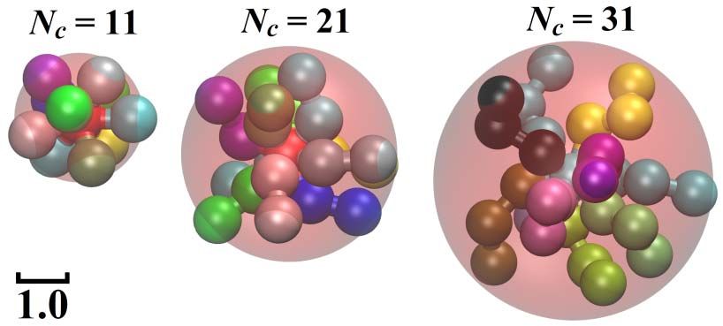
Outline
1.   Background
2.   Fluctuation-dissipation theorem
3.   Kinetic theory
4.   DPD ----> Navier-Stokes
5.   Navier-Stokes ----> (S)DPD
6.   Microscopic ----> DPD
     •   Mori-Zwanzig formalism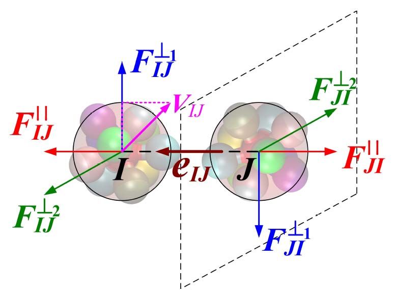
1. Background Molecular dynamics (e.g. Lennard-Jones): – Lagrangian nature – Stiff force – Atomic time step (Allen & Tildesley, Oxford Univ. Press, 1989) Coarse-grained (1980s): Lattice gas automata – Mesoscopic collision rules – Grid based particles (Frisch et al, PRL, 1986)
Mesoscale + Langrangian?
Physics intuition: Let particles represent clusters
of molecules and interact via pair-wise forces
C R
Fi = ∑ Fij + Fij( D
dt + Fij )
j ≠i
Conditions:
– Conservative force is softer than Lennard-Jones
– System is thermostated by two forces
– Equation of motion is Lagrangian as:
dri = v i dt dv i = Fi dt
This innovation is named as DPD method!
Hoogerbrugge & Koelman, EPL, 1992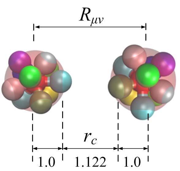
Outline
1.   Background
2.   Fluctuation-dissipation theorem
3.   Kinetic theory
4.   DPD ----> Navier-Stokes
5.   Navier-Stokes ----> (S)DPD
6.   Microscopic ----> DPD
     •   Mori-Zwanzig formalism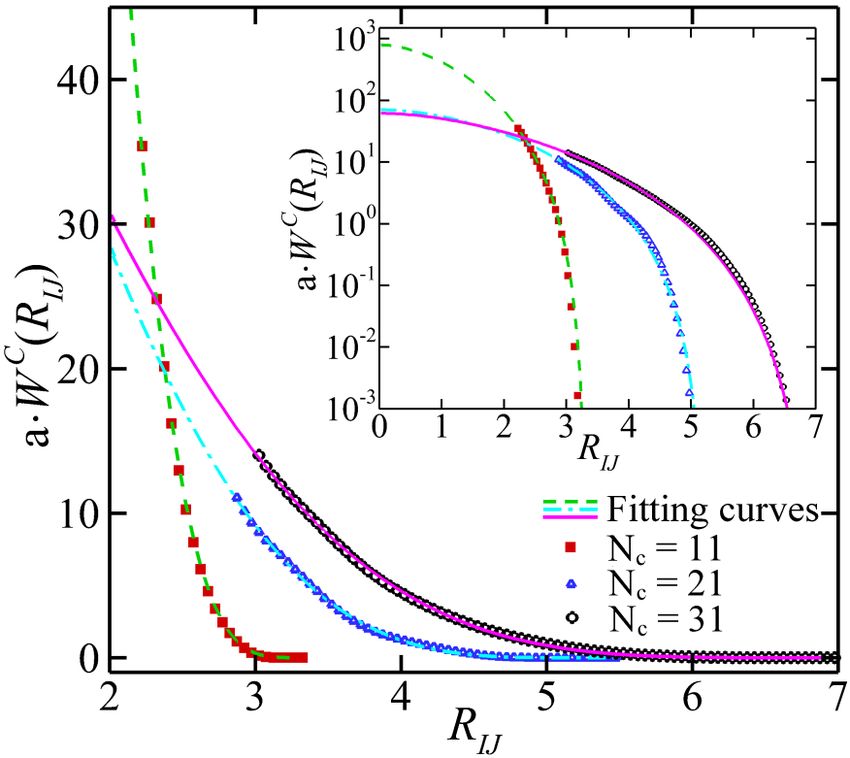
2. Fluctuation-dissipation theorem Langevin equations (SDEs) With the independent Wiener increment: Corresponding Fokker-Planck equation (FPE)

2. Fluctuation-dissipation theorem
Gibbs distribution: steady state solution of FPE
Require Energy dissipation and generation balance
DPD version of fluctuation-dissipation theorem
DPD can be viewed as canonical ensemble (NVT)
Espanol & Warren, EPL, 1995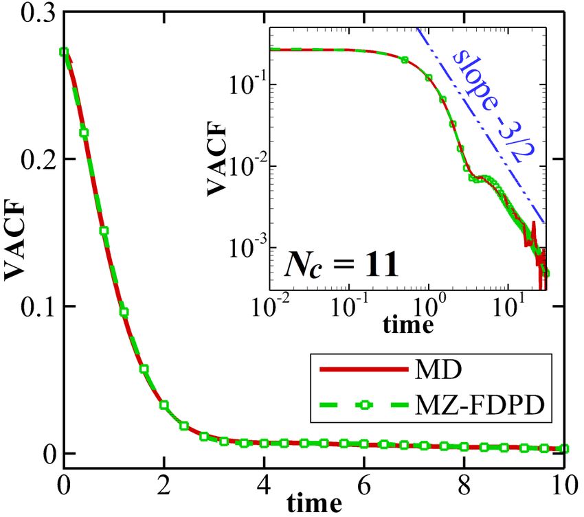
Outline
1.   Background
2.   Fluctuation-dissipation theorem
3.   kinetic theory
4.   DPD ----> Navier-Stokes
5.   Navier-Stokes ----> (S)DPD
6.   Microscopic ----> DPD
     •   Mori-Zwanzig formalism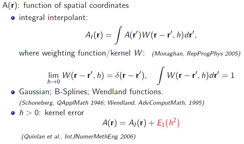
3. Kinetic theory
How to choose simulation parameters?
Strategy: match DPD thermodynamics to atomistic system

    I. How to choose repulsion parameter? (See Lecture I)

            Match the static thermo-properties, i.e.,

                  Isothermal compressibility (water)

                  Mixing free energy, Surface tension (polymer blends)

    II. How to choose dissipation (or fluctuation) parameter?

            Match the dynamic thermo-properties, i.e.,

                  Self-diffusion coefficient, kinematic viscosity
                      (however, can not match both easily)
       Schmidt number             usually lower than atomic fluid
Friction parameters for simple fluids
Simple argument by Groot & Warren, JChemPhys., 1997
Consider an uniform linear flow
Dissipative contribution to stress
Dissipative viscosity
Motion of single particle:
ignore conservative forces, average out other particle velocities
Self-diffusion coefficient
ViscosityKinetic theory:
Fokker-Planck-Boltzmann Equation
Marsh et al, EPL & PRE, 1997
Single-particle and pair distribution functions
Assume molecular chaos
Fokker-Planck-Boltzmann equation
with collision termKinetic theory: dynamic properties
Integration of FPB over v yields continuity equation
Multiplying FPB by v and integrate over v yields momentum equation
kinetic part of the pressure tensor
dissipative part of the pressure tensor
Compare with NS equationOutline
1. Background
2. Fluctuation-dissipation theorem
3. Kinetic theory
4. DPD ----> Navier-Stokes
5. Navier-Stokes ----> (S)DPD
6. Microscopic ----> DPD
• Mori-Zwanzig formalism4. DPD ----> Navier-Stokes
Strategy:
Stochastic differential equations
Mathematically equivalent
Fokker-Planck equation
Mori projection for relevant variables
Hydrodynamic equations
(sound speed, viscosity)
Espanol, PRE, 1995Stochastic differential equations DPD equations of motion
Fokker-Planck equation Evolution of probability density in phase space Conservative/Liouville operator Dissipative and random operators
Mori projection
(linearized hydrodynamics)
Relevant hydrodynamic variables to keep
Equilibrium averages vanishMori projection
Navier-Stokes
Sound speed
Espanol, PRE, 1995Mori projection Stress tensor via Irving-Kirkwood formula: Contributions: Conservative force Dissipative force
Mori projection Viscosities via with Green-Kubo formulas Shear viscosity η and bulk viscosity ζ Projection operator Orthogonal Projection operator Note the squared dependence of viscosity on γ
Outline
1.   Background
2.   Fluctuation-dissipation theorem
3.   Kinetic theory
4.   DPD ----> Navier-Stokes
5.   Navier-Stokes ----> (S)DPD
6.   Microscopic ----> DPD
• Mori-Zwanzig formalism5. Navier-Stokes ---> (S)DPD
Story begins with
smoothed particle hydrodynamics (SPH)
method
Originally invented for Astrophysics
(Lucy. 1977, Gingold & Monaghan, 1977)
Popular since 1990s for physics on earth
(Monaghan, 2005)SPH 1st step: kernel approximation
SPH 2nd step: particle approximation
Error estimated for particles on grid
Actual error depends on configuration of particles
(Price, JComputPhys. 2012)SPH: isothermal Navier-Stokes Continuity equation Momentum equation Input equation of state: pressure and density Hu & Adams, JComputPhys. 2006
SPH: add Brownian motion Momentum with fluctuation (Espanol & Revenga, 2003) Cast dissipative force in GENERIC random force dW is an independent increment of Wiener process
SPH + fluctuations = SDPD Discretization of Landau-Lifshitz’s fluctuating hydrodynamics (Landau & Lifshitz, 1959) Fluctuation-dissipation balance on discrete level Same numerical structure as original DPD formulation
GENERIC framework (part 1)
(General equation for nonequilibrium reversible-irreversible coupling)
Dynamic equations of a deterministic system:
State variables x: position, velocity, energy/entropy
E(x): energy; S(x): entropy
L and M are linear operators/matrices and
represent reversible and irreversible dynamics
First and second Laws of thermodynamics
For any dynamic invariant variable I, e.g, linear momentum
if then
Grmela & Oettinger, PRE, 1997; Oettinger & Grmela, PRE, 1997GENERIC framework (part 2)
(General equation for nonequilibrium reversible-irreversible coupling)
Dynamic equations of a stochastic system:
Last term is thermal fluctuations
Fluctuation-dissipation theorem: compact form
No Fokker-Planck equation needs to be derived
Model construction becomes simple linear algebra
Grmela & Oettinger, PRE, 1997; Oettinger & Grmela, PRE, 1997Outline
1. Background
2. Fluctuation-dissipation theorem
3. Kinetic theory
4. DPD ----> Navier-Stokes
5. Navier-Stokes ----> (S)DPD
6. Microscopic ----> DPD
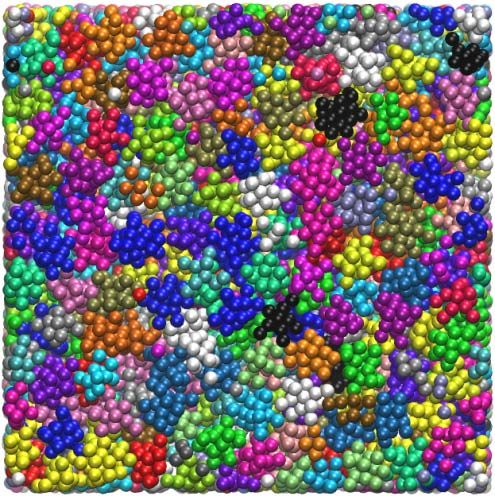
• Mori-Zwanzig formalismCoarse-graining: Voronoi tessellation
Procedure:
1. Partition of particles of molecular dynamics
2. Measuring fluxes at edges
3. Update center of mass
4. Repeat 1, 2 and 3
5. Ensemble average interacting forces
between neighboring Voronoi cells:
similarly as DPD pairwise interactions
Conceptually: useful to support
DPD as a coarse-grained (CG) model
Practically: force fields are useless
and can not reproduce MD system
Flekkoy & Coveney, PRL, 1999Mori-Zwanzig Projection
Mori-Zwanzig Projection
Mori-Zwanzig Projection

Mori, ProgTheorPhys., 1965
Zwanzig, Oxford Uni. Press, 2001
Kinjo & Hyodo, PRE, 2007
MZ formalism as practical tool

Consider an atomistic system consisting of N atoms which
are grouped into K clusters, and NC atoms in each cluster.
The Hamiltonian of the system is:

                   K   NC
                             p 2µ ,i        1
        =H        ∑∑
                  µ  2m
                  = 1 =i 1
                                        +     ∑    ∑
                                            2 µ ,ν i , j ≠i
                                                            Vµi ,ν j
                                 µ ,i

Theoretically, the dynamics of the atomistic system can be
mapped to a coarse-grained or mesoscopic level by using
Mori-Zwanzig projection operators.
The equation of motion for coarse-grained particles can be
written as: (in the following page)
MZ formalism as practical tool
Equation of motion for coarse-grained particles
P = k T ∂ ln ω (R ) Conservative force
µ
∂R µ
B
K
1 Pν ( s )
∑
t
∫
ϑ ϑ
− ds δ F (t − s ) × δ F (0) ⋅
µ ν
T
Friction force
k BT ν =1
0 Mν
+ δ Fµϑ (t ) Stochastic force Kinjo & Hyodo, PRE, 2007
1. Pairwise approximation: Fµ ≈ ∑ µ ≠ν Fµν
2. Markovian approximation: δ Fµϑ (t ) ⋅ δ Fνϑ (0 ) =Γ µν ⋅ δ (t )Coarse-graining constrained fluids
Degree of coarse-graining : Nc to 1
Constrain gyration radius
MD DPD
Atomistic Model Coarse-Grained Model
Coarse
graining
Hard Potential CG Potential
Lei, Caswell, & Karniadakis, PRE, 2010Dynamical properties of constrained fluids
Mean square displacement (long time scale)
Small Rg always fine Large Rg and high density
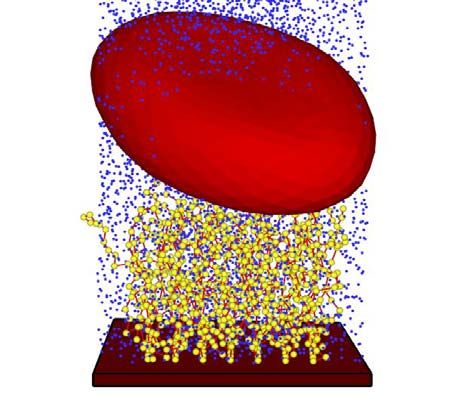
MSD with R g = 0.95 (left) and R g = 1.4397(right)Coarse-graining unconstrained polymer melts
Natural bonds
WCA Potential + FENE Potential
M µ = ∑ mµ ,i
µ ,i
Pµ = ∑ p µ ,i
µ ,i
1
Rµ =
Mµ
∑
µ
mµ rµ
,i
,i ,i
L= ∑ (rµ − R µ ) × (p µ ,i − Pµ )
NVT ensemble with Nose-Hoover
,i
µ ,i
thermostat.Directions for pairwise interactions
between neighboring clusters
1. Parallel direction:
rij= ri − r j
eij = rij / | rij |
2. Perpendicular direction #1:
v=
ij vi − v j
v ij⊥ = v ij − ( v ij ⋅ eij ) ⋅ eij
eij⊥1 = v ij⊥ / | vij⊥ |
3. Perpendicular direction #2:
eij⊥=
2
eij × eij⊥1DPD force fields from MD simulation Conservative Dissipative (parallel one) Li, Bian, Caswell, & Karniadakis, 2014
Performance of the MZ-DPD model (Nc = 11)

     Quantities            MD                 MZ-DPD (error)
      Pressure             0.191               0.193 (+1.0%)
     Diffusivity
                           0.119              0.138 (+16.0%)
 (Integral of VACF)
      Viscosity            0.965              0.851 (-11.8%)
  Schmidt number           8.109              6.167 (-23.9%)
Stokes-Einstein radius     1.155                  1.129 (-2.2%)
Performance of the MZ-FDPD model (Nc = 11)
Quantities MD MZ-FDPD (error)
Pressure 0.191 0.193 (+1.0%)
Diffusivity
0.119 0.120 (+0.8%)
(Integral of VACF)
Viscosity 0.965 0.954 (-1.1%)
Schmidt number 8.109 7.950 (-2.0%)
Stokes-Einstein radius 1.155 1.158 (+0.3%)Conclusion & Outlook • Invented by physics intuition • Statistical physics on solid ground – Fluctuation-dissipation theorem – Canonical ensemble (NVT) • DPD Navier-Stokes equations • Coarse-graining microscopic system – Mori-Zwanzig formalism
You can also read