Does Climate Change Affect Real Estate Prices? Only If You Believe In It - UNEP DTU ...
←
→
Page content transcription
If your browser does not render page correctly, please read the page content below
Does Climate Change Affect Real Estate
                    Prices? Only If You Believe In It
                    Markus Baldauf
                    University of British Columbia

                    Lorenzo Garlappi
                    University of British Columbia

                    Constantine Yannelis
                    University of Chicago

                                                                                                                                      Downloaded from https://academic.oup.com/rfs/article/33/3/1256/5735306 by guest on 14 April 2021
                        This paper studies whether house prices reflect belief differences about climate change.
                        We show that in an equilibrium model of housing choice in which agents derive utility
                        from ownership in a neighborhood of similar agents, prices exhibit different elasticities to
                        climate risk. We use comprehensive transaction data to relate prices to inundation projections
                        of individual homes and measures of beliefs about climate change. We find that houses
                        projected to be underwater in believer neighborhoods sell at a discount compared to houses
                        in denier neighborhoods. Our results suggest that house prices reflect heterogeneity in beliefs
                        about long-run climate change risks. (JEL R31, R32)

                        Received December 7, 2017; editorial decision May 9, 2019 by Editor José Scheinkman.
                        Authors have furnished an Internet Appendix, which is available on the Oxford University
                        Press Web site next to the link to the final published paper online.

                   Introduction
                    Despite broad scientific consensus on the occurrence of climate change, there
                    is substantial disagreement among policy makers and the general public.

                    We thank the editors of the RFS Climate Finance Initiative: Harrison Hong, Andrew Karolyi, and José
                    Scheinkman. We are indebted to two anonymous referees and David Sraer (our discussant). Further, we thank
                    Paul Beaudry, Jonathan Berk, Patrick Bolton, Adlai Fisher, Ralph Koijen, Guangli Lu, Paul Milgrom, Holger
                    Mueller, Vasant Naik, Lubos Pastor, Johannes Stroebel, Raman Uppal, Stijn Van Nieuwerburgh, and Keling
                    Zheng for valuable comments. We are grateful to Krishna Rao, Skylar Olsen, and Lauren Bretz of Zillow
                    Inc. for giving us access to their data and expediting that process. Finally, we thank Dalya Elmalt, Mirko
                    Miorelli, and Emily Zhang for excellent research assistance and Robin Wurl for outstanding support with the
                    NYU Stern Grid computing facility. Baldauf and Garlappi gratefully acknowledge financial support from the
                    Social Science and Humanities Research Council of Canada (SSHRC). This work used the Extreme Science
                    and Engineering Discovery Environment (XSEDE), which is supported by National Science Foundation [ACI-
                    1548562]. Supplementary data can be found on The Review of Financial Studies Web site. Send correspondence
                    to Lorenzo Garlappi, University of British Columbia, Sauder School of Business, 2053 Main Mall, Vancouver,
                    BC, V6T 1Z2, Canada; telephone: 604-822-8848. E-mail: lorenzo.garlappi@sauder.ubc.ca.

                    © The Author(s) 2020. Published by Oxford University Press on behalf of The Society for Financial Studies.
                    All rights reserved. For permissions, please e-mail: journals.permissions@oup.com.
                    doi:10.1093/rfs/hhz073

[16:57 30/1/2020 RFS-OP-REVF190079.tex]                                                                      Page: 1256   1256–1295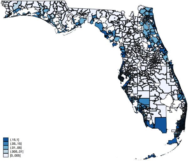
Does Climate Change Affect Real Estate Prices?

                  In March 2017, 42% of Americans surveyed agreed that global warming will
                  pose a serious threat to their way of life, whereas 57% disagreed (Gallup 2017).1
                  Are such differences of opinion reflected in the prices of assets exposed to the
                  consequences of long-run variability of climatic patterns?
                     In this paper we study whether residential real estate prices are affected
                  by differences in beliefs about the occurrence and effects of climate change.
                  Real estate is arguably the ideal asset class to address this question. First, its
                  long-duration nature exposes it to the type of long-run risks that emanate from
                  climate change. Second, real estate is by far the most important asset for the
                  majority of households: the current homeownership rate is 63.6% (U.S. Census
                  Bureau 2017), and the average household holds 40% of its assets in residential
                  property, in contrast to 30.5% invested in financial assets (SCF 2013). Third,
                  real estate is also an important source of household debt, adding to its relevance

                                                                                                                                           Downloaded from https://academic.oup.com/rfs/article/33/3/1256/5735306 by guest on 14 April 2021
                  in the overall economy.
                     One source of risk in the valuation of real estate stems from natural disasters,
                  such as floods, fires, and earthquakes. Such current risks are accounted for in
                  the form of lower real estate valuations or higher insurance premiums, and
                  are already documented in the literature. A largely ignored issue, however, is
                  whether changes in future risks are reflected in real estate valuations. Climate
                  change—that is, the change in the statistical distribution in future weather
                  patterns—falls into this second category of “long-run” risks. In our paper, we
                  investigate the link between differences in expectations about future risks and
                  real estate prices by focusing on changes in flood risk associated with rising sea
                  levels due to climate change. Scientific projections indicate that climate change
                  will lead to a rise in the global sea level and that this will affect the coastal
                  regions in the United States over the coming decades.2 Approximately 2% of
                  U.S. homes—worth a combined $882 billion—are at risk of being inundated
                  by 2100. In some coastal areas, such as Hawaii and Florida, between 10% and
                  12% of all homes are expected to be underwater if sea levels rise by 6 feet (Rao
                  2017).
                     To understand the effect of heterogeneous beliefs on real estate prices and
                  guide our empirical investigation, we build a simple frictionless model of the
                  housing market. Agents differ in their beliefs about the occurrence of climate
                  change and their preferences exhibit homophily, that is, they derive utility from
                  owning a house in a neighborhood populated by like-minded owners. This tie
                  to the community in which agents live acts as a friction for households who
                  plan to leave a homogeneous neighborhood in response to lower home prices
                  elsewhere. If the homophily effect is strong enough, then an equilibrium exists

               1 The media also has highlighted this polarization. A Wall Street Journal article by Newmann (2018) starkly
                  epitomizes this polarization of opinion. The article documents that California localities warn of climate-change-
                  related disaster when suing oil companies, while excluding such risks from the prospectuses of their municipal
                  bonds. Such inconsistencies have led Exxon Mobil to a countersuit.
               2 See, for example, the Digital Coast Data project (National Oceanic and Atmospheric Administration 2018).

                                                                                                                           1257

[16:57 30/1/2020 RFS-OP-REVF190079.tex]                                                                           Page: 1257   1256–1295
The Review of Financial Studies / v 33 n 3 2020
in which “believers” and “deniers” sort into different neighborhoods. In this
“segmented” equilibrium, house prices in different neighborhoods may exhibit
different sensitivities to climate change.
In our empirical analysis we employ three data sources. First, we obtain
scientific forecast data on sea levels from the National Oceanic and Atmospheric
Administration (NOAA). Second, we obtain data on beliefs about climate
change risks from the Yale Program on Climate Change. Third, we employ
proprietary data from Zillow on repeated home transactions for more than ten
million homes, matched to sea-level rise projections.
We employ a hedonic model for house prices that we augment with measures
of climate risks and households’ beliefs about climate change. Our analysis
shows that differences in beliefs about climate change significantly affect house
prices. Specifically, a 1-standard-deviation increase above the national mean in
Downloaded from https://academic.oup.com/rfs/article/33/3/1256/5735306 by guest on 14 April 2021
the percentage of climate change “believers” is associated with an approximate
7% decrease in house prices for homes projected to be underwater. This finding
quantifies the valuation gap between homes in believer and denier counties.
However, it does not speak to the determinants of that difference. The effects
we find may be due to overreaction by believers, underreaction by deniers,
or a combination of both. This result is robust to a wide range of controls
including house characteristics, zoning restrictions, amenities, variation in
climate-change awareness overtime, salience of flood risk, and house supply
effects.
Our work is related to the large literature on heterogeneous beliefs and asset
markets.3 Prompted by the inherent difficulties of homogeneous expectation
models in explaining house price variations through changes in income,
amenity, or interest rates (Glaeser and Gyourko 2006), recent work in real
estate pricing has focused on the role of differences in beliefs (e.g., Burnside,
Eichenbaum, and Rebelo 2016; Piazzesi and Schneider 2009; Favara and Song
2014; Bakkensen and Barrage 2017). Our model builds on the frictionless
competitive equilibrium considered in Burnside, Eichenbaum, and Rebelo
(2016) and introduces agents with a preference for owning in a neighborhood
that is populated by like-minded owners, a property often referred to as
“homophily.”4 Unlike Burnside, Eichenbaum, and Rebelo (2016), who are
3 This literature is too vast to be reviewed here. A common theme emerging from this large body of work is that
in a market-mediated environment, differences in beliefs can lead to speculative trading, bubbles, and excess
volatility (e.g., Miller 1977; Harrison and Kreps 1978; Morris 1996; Scheinkman and Xiong 2003; Kuchler and
Zafar 2017; Bailey et al. 2017, 2018), whereas at the firm level it can lead to overinvestment (e.g., Shleifer and
Vishny 1990; Blanchard, Rhee, and Summers 1993; Stein 1996; Gilchrist, Himmelberg, and Huberman 2005;
Bolton, Scheinkman, and Xiong 2006).
4 The term “homophily” encapsulates the old idea that “birds of a feather flock together.” Lazarsfeld and Merton
(1954) coined the term in the sociological literature to explain a phenomenon that has been found to be a pervasive
and important force in social networks (e.g., McPherson, Smith-Lovin, and Cook 2001; Currarini, Jackson, and
Pin 2009). Favilukis and Van Nieuwerburgh (2017) use a similar mechanism and refer to it as a “consumption
externality.” A subtle difference between our approach and theirs is that in our setting the characteristic that
makes a neighborhood attractive to an agent emerges endogenously, whereas in their setting it is an exogenous
attribute of a location.
1258
[16:57 30/1/2020 RFS-OP-REVF190079.tex] Page: 1258 1256–1295Does Climate Change Affect Real Estate Prices?
interested in the formation and dynamics of housing pricing bubbles, we focus
on the cross-sectional properties of house prices and establish the existence of
equilibria in which market segmentation by beliefs can arise endogenously. This
spatial feature of our equilibrium also distinguishes our work from the literature
of search frictions in the housing market, such as Piazzesi and Schneider
(2009), Favara and Song (2014), and Piazzesi and Stroebel (2015).5 Models
of search frictions can rationalize the empirical fact that transaction volumes
and time to sell are correlated with average house prices. We abstract away
from this generalization which is tangential to the focus of our study. Unlike
our model, which features two marginal agents in two different neighborhoods,
both Piazzesi and Schneider (2009) and Favara and Song (2014) feature search
models with optimistic marginal buyers only. As in our model, in Piazzesi
and Stroebel (2015) house prices are determined in equilibrium by different
Downloaded from https://academic.oup.com/rfs/article/33/3/1256/5735306 by guest on 14 April 2021
marginal buyers. However, while Piazzesi and Stroebel (2015) use a search
model to study the equilibrium effect of buyers with different search “breadth,”
we rely on a competitive equilibrium model to obtain endogenous valuations
of neighborhoods when agents have heterogeneous beliefs.
Our work is also related to the nascent and growing literature concerned
with the effects of climate change and asset markets. Relevant contributions to
this literature include Giglio et al. (2015), Gibson, Mullins, and Hill (2017),
Lemoine (2017), and Hong, Li, and Xu (2019). Giglio et al. (2015) study
discount rates for valuing investments in climate change abatement. They find
low discount rates to be appropriate at all horizons. They also use Zillow data
and NOAA maps, and identify properties that will be flooded with a 6-foot rise
in sea levels. They construct a climate attention index using textual analysis
and find that when the fraction of listings that mention climate change doubles,
properties projected to be flooded relative to other properties decrease by 2% to
3%. Gibson, Mullins, and Hill (2017) make explicit the link between new flood
maps and the beliefs of agents and connect this to regular price signals, such as
the cost of insurance. Lemoine (2017) distinguishes between direct “weather”
(current risks) and “climate” (long-run distribution of weather) channels to
study their implications for economic outcomes in a dynamic setting with
rational expectations. Our study builds on this literature by not only focusing
on the relationship of home prices and current risks but also expected future
changes in flood risk. Variation in our data allows us to test the link between
current market prices and belief heterogeneity controlling for current risks, as
well as projections about future risks.
A closely related paper is Bakkensen and Barrage (2017), who study the
effect of difference in beliefs about climate risk on the selection choice
between coastal and noncoastal homes. Using a similar model as Burnside,
Eichenbaum, and Rebelo (2016) with Bayesian learning, they show that
5 Burnside, Eichenbaum, and Rebelo (2016) also analyze a search and matching model along the lines of Piazzesi
and Schneider (2009).
1259
[16:57 30/1/2020 RFS-OP-REVF190079.tex] Page: 1259 1256–1295The Review of Financial Studies / v 33 n 3 2020
heterogeneity in beliefs dramatically increases the projected housing market
impact of future flood risk. In particular, if a fraction of agents are misinformed
about sea-level rise and learn about it by observing current storms, then
these agents can lead to overvaluations, excess volatility and sharp price
decline as flood risk rises. Based on survey evidence from Rhode Island,
Bakkensen and Barrage (2017) show that coastal residents attach higher
amenity values to coastal living and lower flood risk perceptions, relative to
inland owners. Our work differs from theirs along several dimensions. First,
we focus on the price differences within otherwise identical coastal properties
and do not consider the location choice between coastal and noncoastal regions.
Second, their agents differ in their individual-specific amenity value that they
derive from coastal owning. In contrast, our agents, have a “network-specific”
amenity value (homophily). This allows us to construct an equilibrium in
Downloaded from https://academic.oup.com/rfs/article/33/3/1256/5735306 by guest on 14 April 2021
which two otherwise identical coastal neighborhoods have marginal buyers
with different beliefs about climate change (i.e., we do not rely on exogenous
variation of characteristics). Third, our empirical analysis focuses on a much
larger sample of transaction-level real estate prices, which we combine with
NOAA projections on sea-level rise and national-level survey data from the Yale
Climate opinion project. Finally, the findings in Bakkensen and Barrage (2017)
are primarily about the salience of current extreme weather events, while our
focus is on the effect of difference in beliefs about future events resulting from
long-run changes in climate patterns.
Our work is also related to contemporaneous work by Bernstein, Gustafson,
and Lewis (2018), who estimate a discount in home prices of 7% due to exposure
to sea-level rise. They find that this difference is more pronounced for non-
owner-occupied properties, which they interpret as a reflection of increased
sophistication of their owners. While their focus is mainly on estimating the
price effect of sea-level rise, Bernstein, Gustafson, and Lewis (2018) also use
data from the Yale Climate opinion survey to find that belief differences only
affect the price of sea-level rise exposure in the owner-occupied segment of
the market. We differ from this study along two dimensions. First, the main
analysis of Bernstein, Gustafson, and Lewis (2018) focuses on assessing the
effect of sea-level rise on house prices. In contrast, our focus is on the effect
of differences in beliefs about sea-level rise on house prices. Second, we
provide a theoretical framework that helps shape our empirical analysis on
the effect of beliefs about climate change on house prices. Consistent with our
results, Bernstein, Gustafson, and Lewis (2018) find that beliefs about climate
change are important in the pricing of owner-occupied coastal properties. They
show that exposed homes located in counties where agents are most worried
about climate change sell at a 8.5% discount. This estimate is comparable
to the 7% discount in our analysis. Furthermore, their interpretation—
that beliefs about climate change matter most when owners themselves
occupy the home—is consistent with our mechanism based on homophily in
homeownership.
1260
[16:57 30/1/2020 RFS-OP-REVF190079.tex] Page: 1260 1256–1295Does Climate Change Affect Real Estate Prices?
Finally, our work also relates to contemporaneous work by Murfin and
Spiegel (2018). They focus on estimating the effect of sea-level rise on house
prices, rather than heterogeneity in beliefs. Murfin and Spiegel (2018) use
comprehensive data on coastal home sales and data on elevation relative to
local high tides, whose variation they leverage in their estimation. In contrast
to our findings, Murfin and Spiegel (2018) find an upper bound for the projected
effects of sea-level rise on real estate prices that is quite small. The difference
relative to our results is likely due to two factors. First, Murfin and Spiegel
(2018) focus on an average effect while in our analysis we focus on how this
effect varies with beliefs. Second, they exploit a different source of variation
of sea-level rise resulting from vertical land motion. Areas with vertical land
motion leading to higher projected sea-level rise tend to be in areas with more
climate change deniers, such as Texas and Louisiana, where our model would
Downloaded from https://academic.oup.com/rfs/article/33/3/1256/5735306 by guest on 14 April 2021
suggest smaller effects of projected sea-level rise. Thus, we do not view their
results as being inconsistent with belief heterogeneity affecting the impact of
projected sea-level rise on real estate prices.
1. Model
We consider a simple frictionless model of the housing market in which
agents may differ in their beliefs about the occurrence of climate change. We
assume that agents have preferences that exhibit “homophily,” that is, they
derive utility from owning houses in a neighborhood populated by like-minded
owners. Because of homophily, agents have strong ties to the community in
which they live, and this acts as a friction for households who plan to leave
a homogeneous neighborhood in response to lower home prices elsewhere.
Under the conditions we specify below, we show the existence of equilibria in
which “believers” and “deniers” sort themselves into geographically identical
neighborhoods. Furthermore, we show that equilibrium house prices may differ
in their sensitivity to climate change risk.
1.1 Setup
We consider a discrete-time, infinite-horizon, model economy populated by
a continuum of agents with measure one divided into a mass μb ∈ [0,1] of
climate change “believers,” and a mass μd = 1−μb of climate change “deniers.”
Believers and deniers disagree on the likelihood of climate-related events, for
example, sea-level rise. We refer to believers as agents who attach a larger
probability to climate-related events than deniers. All agents have linear utility
with constant discount rates β h , h ∈ {b,d}. Agents can either own a house or
rent.
There is a fixed stock of houses, k < 1, split in two geographically identical
neighborhoods.6 The rental market is composed of 1−k units produced by
6 The fixed supply assumption is common in the literature, and it has been justified by the presence of zoning laws,
land scarcity, or infrastructure constraints (e.g., Burnside, Eichenbaum, and Rebelo 2016).
1261
[16:57 30/1/2020 RFS-OP-REVF190079.tex] Page: 1261 1256–1295The Review of Financial Studies / v 33 n 3 2020
competitive firms at a cost, the rental rate, that, without loss of generality, we
normalize to zero.
Agents’ utility from owning in a neighborhood increases in the number of
similar types that own in the same neighborhood. We refer to the positive effect
of owning in like-minded neighborhoods as homophily. The expected utility of
an agent of type h ∈ {b,d} in neighborhood n ∈ {1,2} is
Unh = ε h +φ(μhn ), (1)
h
where ε is agent h’s per-period expected utility from owning, μhn
is the mass
of type-h agents owning in neighborhood n, and φ(·) is a weakly increasing
function representing homophily. The larger the mass μhn of type-h agents in
neighborhood n, the larger agent h’s utility from owning a house in n. We
normalize the homophily function to φ(0) = 0.
Downloaded from https://academic.oup.com/rfs/article/33/3/1256/5735306 by guest on 14 April 2021
1.2 Equilibrium
Let μhn ≤ μh be themass of h-owners, h ∈ {b,d}, in neighborhood n ∈ {1,2},
and let μhR = μh − n μhn be the mass of h-renters. We define a pair (μb ,μd )
as an allocation of b- and d-homeowners, where the triplet μh = (μh1 ,μh2 ,μhR )
contains the mass of type-h agents in neighborhoods 1, 2, and rental housing.
An allocation is feasible if, for h ∈ {b,d} and n ∈ {1,2}, μhn ≥ 0 and μhR ≥ 0.
Equilibrium house prices in neighborhood n are determined by the marginal
buyer h in that neighborhood. Such a buyer will be indifferent between buying
h
a home in neighborhood n and renting. The price Pn,t that makes agent h
indifferent between owning in area n and renting is given by
−Pn,t
h
+β h (ε h +φ(μhn )+Eh [Pn,t+1 ]) = 0, h ∈ {b,d}, n ∈ {1,2}, (2)
where Pn,t+1 denotes the prevailing price at time t +1. If h is the marginal buyer
in neighborhood n, the indifference price Pnh in a stationary equilibrium is given
by the nonexplosive solution of (2), that is,
βh
Pnh = (ε h +φ(μhn )), h ∈ {b,d}, n ∈ {1,2}. (3)
1−β h
A competitive equilibrium in the housing market is represented by a set of house
prices in the two neighborhoods, (P1 ,P2 ), and a set of allocations (μb ,μd ) such
that the house market clears. In a segmented equilibrium, the marginal buyer in
neighborhood n is different from the marginal buyer in the other neighborhood.
Because deniers attach a smaller probability to climate-related events than
believers, deniers’ per-period expected utility from owning, ε d , is larger than
believers’, εb . We assume that the same valuation hierarchy holds for the
perpetuity value of owning a home. Specifically,
Assumption 1 (Valuation hierarchy). In the absence of homophily, deniers
value houses more than believers
βd d βb b
d
ε > ε . (4)
1−β 1−β b
1262
[16:57 30/1/2020 RFS-OP-REVF190079.tex] Page: 1262 1256–1295Does Climate Change Affect Real Estate Prices?
One way to interpret Assumption 1 is that agents may disagree about the
random time T after which homes will be permanently flooded, but that they
are otherwise identical, that is, ε d = ε b , β d = β b , and εth = 0 for all t ≥ T . If T
is geometrically distributed, then Assumption 1 implies that the distribution
of the flood arrival time T of believers dominates that of deniers in a first-
order sense. To see this, suppose that ρ denotes the common discount rate,
ε the common expected utility from owning, and that Ph [T ≤ t] = 1−γht+1 ,
t ∈ {0,1,2...}, where γh ∈ (0,1] denotes the agent-specific survival probability.
Then, in the absence of homophily, agent’s h’s valuation is
T ∞
Eh t
ρε = Ph [T ≥ t]ρ t ε
t=1 t=1
Downloaded from https://academic.oup.com/rfs/article/33/3/1256/5735306 by guest on 14 April 2021
∞
ργh
= Ph [T > t −1]ρ t ε = ε (5)
t=1
1−ργh
The above expression illustrates that the discount factor β h in Assumption 1
can be thought of as the product of a common time-preference parameter ρ and
a survival probability parameter γh . Assumption 1 implies that γb < γd , that is,
believers attach a lower probability of survival than deniers.
We further assume that the homophily effect from owning a house is
sufficiently strong, specifically,
Assumption 2 (Homophily). The homophily benefit perceived by agent h ∈
{b,d} when the entire neighborhood is composed of type-h agents is such that
β d 1−β b
φ(k/2) ≥ εd −ε b , ≡ . (6)
1−β d β b
Note that if β b = β d , then Assumption 2 requires that the homophily benefit
from owning in a homogeneous neighborhood exceeds the difference ε d −ε b
in the per-period expected utility of owning between the two types of agents.7
The following proposition establishes the existence of a segmented equilibrium
in the housing market.
Proposition 1 (Segmented Equilibrium). If Assumptions 1 and 2 hold and
μb ∈ [k/2,1−k/2], then there exists a stationary segmented equilibrium in
which house prices are given by
βb b
P1 = b
ε +φ(k/2) (7)
1−β
βd d
P2 = d
ε +φ(k/2) (8)
1−β
7 If β b ≤ β d , ≥ 1. Therefore, when believers discount the future more heavily, Assumption 2 imposes a more
stringent requirement on the homophily function φ .
1263
[16:57 30/1/2020 RFS-OP-REVF190079.tex] Page: 1263 1256–1295The Review of Financial Studies / v 33 n 3 2020
and allocations μh = (μh1 ,μh2 ,μhR ) are
μb = (k/2,0,μb −k/2), μd = (0,k/2,1−μb −k/2). (9)
Proposition 1 establishes the existence of an equilibrium in which housing
markets are segmented by type. The result arises because the marginal home
buyer in the two neighborhoods is of a different type. Believers are indifferent
between owning in the believers neighborhood and renting, and deniers are
indifferent between owning in the deniers neighborhood and renting.
1.3 Comparative statics
To analyze the effect of differences in beliefs on the equilibrium prices of
Proposition 1, we need to put some structure on the beliefs of agents. We denote
Downloaded from https://academic.oup.com/rfs/article/33/3/1256/5735306 by guest on 14 April 2021
by s a random variable representing the sea-level rise in a neighborhood whose
distribution is given by P.8 Believers and deniers differ in their assessment of
their subjective distribution Ph of sea-level rise. Specifically, we assume that
agent h’s expected utility from owning depends on the expected sea-level rise
as follows:
ε h = ε −Eh [s] = ε −ξ h EP [s], h ∈ {b,d} (10)
where Eh denotes the expectation under belief Ph , ε represents the utility
from owning regardless of expected sea-level rise, and constant ξ h denotes
the sensitivity of agent h’s expected utility to sea-level rise.9 Believers differ
from deniers in that they attach higher probability to higher values of sea-level
rise s. The following assumption formalizes the condition on the differences in
beliefs.
Assumption 3 (Difference in Beliefs). The sensitivities ξ b and ξ d of agents’
expected utilities to changes in sea level rise satisfy:
ξ b ≥ ξ d . (12)
When β b < β d , ≥ 1 (see footnote 7), the above assumption requires that
believers have to be sufficiently more sensitive than deniers to changes in sea-
level rise. The following proposition characterizes the sensitivity of equilibrium
prices from Proposition 1 to expected sea-level rise.
8 One possible interpretation is to think of P as the “objective” distribution, based on climate science models.
9 In general, one can think of the sensitivity ξ h in (10) as a random variable representing a change of measure
d Ph /d P > 0. In this case, ξ h can be used to define agent h’s expectation as follows
h
EP [s] = EP [ξ h s], h ∈ {b,d}. (11)
In this setting, the analog to Assumption 3 would be to require that the ratio ξ b (s)/ξ d (s) is increasing in s (that is,
it satisfies the monotone likelihood ratio property, MLRP). By MLRP, ξ b first-order stochastically dominates ξ d
b d
and therefore EP [s] ≥ EP [s]. From the definition of agents’ expected utility (10) we deduce that this condition
is conceptually equivalent to Assumption 3.
1264
[16:57 30/1/2020 RFS-OP-REVF190079.tex] Page: 1264 1256–1295Does Climate Change Affect Real Estate Prices?
Downloaded from https://academic.oup.com/rfs/article/33/3/1256/5735306 by guest on 14 April 2021
Figure 1
Model’s prediction
This figure plots house prices of Proposition 1 against expected sea-level rise. Because the conditions of
Proposition 2 are satisfied, home prices in the believer neighborhoods are more sensitive to changes in the expected
sea-level rise than are home prices in denier neighborhoods. We use the following parameters: β b = β d = 0.993,
ξ b = 1, ξ d = ξ b /2, ε = 1, and φ(k/2) = 1.
Proposition 2 (Comparative Statics). Let S ≡ EP [s] denote the expected sea-
level rise under measure P. Under assumptions 1, 2, and 3, the equilibrium prices
of Proposition 1 have weakly increasing differences in S, that is,
P1 (S)−P1 (S ) ≥ P2 (S)−P2 (S ), for S > S. (13)
Figure 1 illustrates the comparative statics result of Proposition 2. The main
empirical prediction of the model is that if (a) deniers value houses more than
believers (Assumption 1), (b) homophily is sufficiently strong (Assumption 2)
and (c) believers are more sensitive to news about sea-level rise (Assumption 3),
then, in equilibrium, the elasticity of house prices to sea-level rise is higher
in believers’ neighborhood than in deniers’ neighborhood. In the analysis
of Section 3 we assess the validity of the comparative statics described in
Proposition 2 by empirically analyzing the effect of belief heterogeneity about
climate change on real estate prices in the United States.
2. Data
In this section we describe the data sources and the construction of our main
analytic data set. Table 1 contains a summary description of the variables we use
in our analysis. We rely on three main data sources: (a) transacted home values
1265
[16:57 30/1/2020 RFS-OP-REVF190079.tex] Page: 1265 1256–1295The Review of Financial Studies / v 33 n 3 2020
Table 1
Variable descriptions
Name Description Source
Pit Dollar transaction price of home i at time t Zillow
UnderWateri Indicator of whether home i is located in an area that is Zillow
projected to be affected by sea level inundation of 6 ft.
above current Mean Higher High Water (MHHW) by
2100, based on NOAA projections
Hc Percentage of residents in county c who answered “Yes” HMMLa
to the Yale Climate Survey question: “Do you think that
global warming is happening?”
Regional controls
Income Adjusted gross income (AGI) at zip code level (in 1,000 IRSb
USD) for 2014
Temperature Daily Air Temperatures and Heat Index (1979–2011) NLDASc
Flood 10 y Height of a flood (in cm) that has a ten percent chance CC/NOAAd
of occurring in a given year, for each NOAA station
Downloaded from https://academic.oup.com/rfs/article/33/3/1256/5735306 by guest on 14 April 2021
(https://water.usgs.gov/edu/100yearflood.html)
Population Population count (in thousands) for each zip code ACSe
Elevation Elevation (in meters) at the centroid of each zip code Google
(2018)
GOP share Percentage of individuals in a zip code voting for the HEDAf
Republican Party
House controls
Age Age of the property (in years) ZTRAX
Year built Year the property was built ZTRAX
Size Area of the building (in sq.ft.) ZTRAX
Number of bedrooms Count of the number of bedrooms of a property ZTRAX
Number of bathrooms Count of the number of bathrooms of a property ZTRAX
Garage Indicator for whether a property has a garage ZTRAX
Agricultural Zoning indicator: Agricultural use ZTRAX
Communication Zoning indicator: Communication use ZTRAX
Commercial Zoning indicator: Commercial use ZTRAX
Exempt & institutional Zoning indicator: Public use ZTRAX
Governmental Zoning indicator: Governmental use ZTRAX
Industrial Zoning indicator: Industrial use ZTRAX
Industrial-heavy Zoning indicator: Industrial-heavy use ZTRAX
Historical & cultural Zoning indicator: Historical and cultural use ZTRAX
Miscellaneous Zoning indicator: Miscellaneous use ZTRAX
Personal Zoning indicator: Personal use ZTRAX
Recreational Zoning indicator: Recreational use ZTRAX
Multifamily Zoning indicator: Multifamily use ZTRAX
Residential Zoning indicator: Residential use ZTRAX
Transportation Zoning indicator: Transportation use ZTRAX
Vacant Indicator for whether land is vacant ZTRAX
Distance Distance of a property to the closest coast line Authors’
calculations
Neighborhood density Number of properties within a 0.5-km radius Authors’
calculations
Amenity controls
Income Adjusted gross income (AGI) at the ZIP code level (in IRSb
1,000 USD) for 2014
Temperature Daily Air Temperatures and Heat Index (1979–2011) NLDASc
Population Population count (in thousands) for each ZIP code ACSe
Latitude/longitude Geographical coordinates of a property ZTRAX
Education Share of individuals with a bachelor’s degree in 2015 ACSe
a Howe et al. (2015)
b Internal Revenue Service
c North America Land Data Assimilation System (NLDAS), https://wonder.cdc.gov/nasa-nldas.html
d Climate Central (CC) and National Oceanic and Atmospheric Administration (NOAA)
e American Community Survey (ACS)
f Harvard Election Data Archive (HEDA), https://projects.iq.harvard.edu/eda/data
1266
[16:57 30/1/2020 RFS-OP-REVF190079.tex] Page: 1266 1256–1295Does Climate Change Affect Real Estate Prices?
and characteristics; (b) measures of the projected effects of climate change;
and (c) measures of beliefs about climate change. In what follows we briefly
describe the data used in our analysis. Table 1 lists all of the variables used,
and Appendix B contains a detailed description of the data and various steps
taken to transform the raw data into an analytic data set.
2.1 Real estate
Our main sources of real estate data are transactions data and proprietary
supplemental data from Zillow Inc. Specifically, we use the Zillow Transaction
and Assessment Data Set (“ZTRAX”), which Zillow provides to qualifying
academic and institutional researchers. The Zillow transaction data has a 20-
year history of property transactions from 1997 to 2017, as well as detailed
Downloaded from https://academic.oup.com/rfs/article/33/3/1256/5735306 by guest on 14 April 2021
home characteristics from more than 374 million public records across over
2,750 counties. Furthermore, Zillow provides us with a proprietary data set
that contains home valuations based on their Zestimate algorithm as well as
proprietary geographic information that can be used to match individual homes
to future flood zones.
These data sets contain information about the geographic location for each
home as well as a host of house-specific characteristics, such as size, availability
of parking, number of rooms and bathrooms, that we use both as controls and
as determinants of the amenity value of a property. We use the geographic
location to match each home to a ZIP code, census tract, or county and to
compute the distance of each home from the coast. Table 1 describes the main
housing variables that we employ.
2.2 Climate
We use two types of climate change variables: (1) variables that describe the
current climate and (2) variables pertaining to the change in climate. We start
from publicly available maps by NOAA, which show the mean higher high
water (MHHW) tidal datum, using a 6-foot sea-level rise above the current
level. NOAA defines the tidal datum MHHW as the best possible approximation
of the threshold at which inundation can begin to occur.10 Therefore, coastal
homes located below the MHHW level are either permanently submerged under
water or in the intertidal zone, which is typically uninhabited. Zillow constructs
an indicator variable for every home, UnderWater i , that evaluates to unity if
the home falls in a future flood zone.
Variables pertaining to the current state of climate include (a) a measure of
the distance to the coast; and (b) a measure of the current risk of an extreme
flood that has a 10% probability of occurring (Flood 10 y).
10 The mean higher high water is the average of the higher high water height of each tidal day observed over the
National Tidal Datum Epoch (National Oceanic and Atmospheric 2013).
1267
[16:57 30/1/2020 RFS-OP-REVF190079.tex] Page: 1267 1256–1295The Review of Financial Studies / v 33 n 3 2020
2.3 Beliefs about climate change
The main data source to measure beliefs about climate change is the Yale
Climate Opinion Maps 2016 (Howe et al. 2015). This study provides, at the
county level, survey evidence of how respondents answer questions, including
(a) whether they believe that climate change is happening; (b) whether they
believe that climate change is human caused; (c) whether they believe that
there is scientific consensus on whether climate change is happening; and (d)
whether they will be personally affected by climate change. Our main measure
of beliefs in climate change is the percentage Hc of people who answered “Yes”
to survey question (a).
2.4 Control variables
Downloaded from https://academic.oup.com/rfs/article/33/3/1256/5735306 by guest on 14 April 2021
We employ a number of variables to control for local conditions in our analysis.
Specifically, control variables at the ZIP code level include demographic
variables, such as population, income, and political voting measures, that relate
to the geography of a ZIP code, such as elevation at the centroid, current
flood risk, and weather. To control for the amenity value of a home, we follow
the procedure of Albouy (2016). We discuss the construction of the amenity
measure in footnote 15. We also directly construct house-level measures of
amenity and zoning variables from the Zillow data.
2.5 Data construction
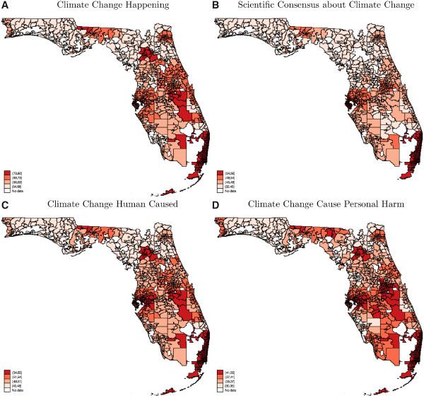
We restrict attention to homes located within a distance of 50 km from the
coast.11 Across these homes there is considerable variation in (a) the impact
of sea-level rise; and (b) the beliefs of residents about climate change. For
example, Figure 2 shows the fraction of homes projected to be underwater given
a 6-foot sea-level rise in Florida ZIP codes, and Figure 3 reports the fraction of
people agreeing with the statement that climate change is happening in the Yale
Climate Survey regarding climate change for Florida ZIP codes. Both figures
show considerable variation along these two dimensions across ZIP codes.
Table 2 reports the summary statistics of the variables used in our regression
analysis. The average house price in our sample is $286,130 (median $190,000).
On average 8.5% of properties are located in a future flood zone and an average
of 72.32% of households answered “Yes” to the Yale Climate Opinion Survey
question: “Do you believe that climate change is happening?”
3. Empirical Analysis
3.1 Methodology
The key empirical challenge we face is that home valuations may vary along
dimensions other than their projected exposure to sea-level rise and the degree
11 The Online Appendix, Table OA.2, shows that these results are not sensitive to this restriction.
1268
[16:57 30/1/2020 RFS-OP-REVF190079.tex] Page: 1268 1256–1295Does Climate Change Affect Real Estate Prices?
Downloaded from https://academic.oup.com/rfs/article/33/3/1256/5735306 by guest on 14 April 2021
Figure 2
Underwater homes in Florida
This figure shows the fraction of homes projected to be underwater given 6 feet of sea-level rise in Floridan ZIP
codes. National parks and lakes are excluded. Source: NOAA.
of belief in climate change of the neighborhood in which the property is located.
For example, homes closer to the coast may be more likely to face damage in
the event of sea-level rise, but at the same time they may be more valuable
due to coastal views. We address this concern by specifying a hedonic pricing
model that controls for individual building characteristics, such as distance
from the coast, and attributes of neighborhoods, such as neighborhood density
and average temperature.
Our main dependent variable is the natural logarithm of the transaction price
of home i at time t, lnPit . The independent variables fall into the following
categories: (a) covariates at the home level that encompass an indicator for
whether home i is projected to be inundated in the future, UnderWateri ,12
and other characteristics of homes, Xi ; (b) covariates at the county level
that include the logarithm of the percentage of residents in a given county
c, who answered “Yes” to the Yale Climate Survey question: “Do you think
that global warming is happening?”, lnHc ; and (c) covariates at the ZIP code
12 Formally, UnderWater is an indicator of whether property i is located in an area projected to be affected by
i
sea-level inundation of 6 feet above current mean higher high water (MHHW) by the year 2100, based on publicly
available NOAA projections.
1269
[16:57 30/1/2020 RFS-OP-REVF190079.tex] Page: 1269 1256–1295The Review of Financial Studies / v 33 n 3 2020
Downloaded from https://academic.oup.com/rfs/article/33/3/1256/5735306 by guest on 14 April 2021
Figure 3
Beliefs about climate change in Florida
This figure shows the fraction of people agreeing with particular statements about climate change in Floridan ZIP
codes. A statement is denoted above each panel. National parks and lakes are excluded. Source: Yale Climate
Opinion Survey.
level, Xz . Our main specification consists of a rich hedonic model of house
prices, which we augment with measures of climate risks and households’
beliefs about climate change. The key identifying assumption is that unobserved
determinants of home prices are uncorrelated with beliefs and whether a home
is underwater, conditional on observables. The main challenge is that, all
else being equal, coastal homes are more valuable than other homes. Thus,
controlling for distance from the coast is particularly important. If, on the one
hand, homes closer to the coast tend to have higher values, on the other hand,
homes closer to the coast are also more likely to be flooded if sea levels rise.
Additionally, if wealthy people live near the coast these homes may also have
different characteristics. For example, these homes may be larger, or newer.
This presents an omitted variable problem which is solved by controlling for
distance from the coast.
We address this issue primarily by controlling for observables. To identify
our effect we include in our hedonic regression (a) geography by distance
from the coast fixed effects; (b) several characteristics that correlate with
1270
[16:57 30/1/2020 RFS-OP-REVF190079.tex] Page: 1270 1256–1295Does Climate Change Affect Real Estate Prices?
Table 2
Summary statistics
Mean Median SD Min Max
Pit 286,129.6 190,000 88,8762.5 1,000 4,750,000
UnderWateri .085 0 .279 0 1
Hc .7232 .7231 .0502 .5609 .8404
Regional & Amenity controls
Income 66,208.97 61,364 66,208.97 19,665 218,152
Temperature 54.554 51.83 9.928 33.95 70.9
Flood 10 y .8395 .7925 1599 .4267 1.341
Population 52,941.61 52,941.61 248,686.8 0 6,557,746
Elevation 50.548 23 76.531 0 1917
GOP share .475 .479 .178 0 1
Amenity .1562 .1301 .2478 -.4039 .8088
Neighborhood density 627.3222 481.0000 612.0047 1 9,934
Downloaded from https://academic.oup.com/rfs/article/33/3/1256/5735306 by guest on 14 April 2021
House controls
Year built 1975 1981 27.412 1586 2017
Size 1,616.097 1427 774.368 1 4,680
Number of bedrooms 2.065 2 1.465 0 5
Number of bathrooms 1.761 2 1.117 0 5
Garage .856 1 .3510 0 1
Observations 11,538,986
This table presents summary statistics for the main analysis variables. Table 1 provides descriptions of the
variables.
flood projections; and (c) interaction terms between flood projections and
county-level characteristics that may correlate with beliefs in climate change.
Specifically, our main regression specification, which we estimate on the full
sample is
lnPit = αzd +αy +ζ UnderWateri ×lnHc +γ Xi
+λ (UnderWateri ×Xi )+ω (UnderWateri ×Xz )+εit , (14)
where αzd denotes ZIP code×distance fixed effects, that vary by ZIP code, and
distance of a home from the coast,13 and αy is a set of year fixed effects, which
evaluate to unity if the transaction date t of home i is in year y.
In addition, we also consider the following specification
lnPit = αced +αy +βUnderWateri +γ Xi +ξ Xz + it , (15)
where αced denotes county×elevation×distance fixed effects, that vary by
county, elevation at the ZIP code’s centroid, and distance of a home from
the coast. We estimate (15) for believer counties (i.e., counties for which Hc ≥
median(Hc )) and denier counties (i.e., counties for which Hc < median(Hc ))
separately.
The main coefficient of interest is ζ in regression (14). This coefficient
captures the elasticity of house prices with respect to beliefs about climate
13 In some specifications, we will instead include county×elevation×distance fixed effects, α
ced .
1271
[16:57 30/1/2020 RFS-OP-REVF190079.tex] Page: 1271 1256–1295The Review of Financial Studies / v 33 n 3 2020
change for an underwater property. In some specifications, we also include
interactions between UnderWateri and hedonic home level controls Xi as well
as geographic controls Xz . To address potential serial correlation, we cluster
standard errors at the county level, which is the level of variation in beliefs.
Using the logarithm variable lnHc , has the attractive property that, without
additional interactions (λ ×Xi and ω ×Xz ), when UnderWateri evaluates to
unity, the term ζ ×UnderWateri can be interpreted as the elasticity of house
price with respect to Hc .
The key identifying assumption is that the error terms εit and it have zero
conditional expectation. An empirical challenge is that the amenity value of
a home may be correlated with Hc . For example, beachfront property may
be more valuable in the South, where more climate change deniers live. Thus,
along with controlling for distance from the coast, it is crucial to include hedonic
Downloaded from https://academic.oup.com/rfs/article/33/3/1256/5735306 by guest on 14 April 2021
controls, Xi and Xz , to explain variation in home prices. We now turn to the
precise definition of these covariates.
3.1.1 Home-level covariates, Xi . We include the distance from the coast
for each home. In addition, following Giglio, Maggiori, and Stroebel (2014),
we include housing characteristics, such as the lot size, number of bedrooms
and bathrooms, parking, age of the property, and distance to the coast.14
Appendix B.3 details how we determined the closest distance of a property
to the coastline. Depending on the specification, we include interaction terms
between these control variables and the UnderWateri indicator.
3.1.2 ZIP-code-level covariates, Xz . The purpose of ZIP-code-level controls
is to account for variables that affect the amenity value of a house, such
as the quality of a neighborhood or the distance from the coast. We
include demographic variables, such as population, income, and political
voting measures. Beliefs about climate change may be correlated with other
determinants of housing prices. For example, Democrats may be more likely
to believe in climate change, but a Democrat controlled area may be following
different land use and zoning policies, which could affect home prices. Short-
term flood risk also may be correlated with homes being projected to be
underwater in the future and depress home prices.
Moreover, people in urban areas may be more likely to believe that climate
change is happening, and home prices may be higher due to geographic
constraints, lower housing supply or the amenity value of living in urban areas.
We also include variables that relate to the geography of a ZIP code, such as
elevation at the centroid, current flood risk, weather, as well as controls for the
amenity value. Finally, we also apply the method described in Albouy (2016),
which develops a measure for the amenity value based on an equilibrium model
14 Table 1 reports the precise list of housing characteristics.
1272
[16:57 30/1/2020 RFS-OP-REVF190079.tex] Page: 1272 1256–1295Does Climate Change Affect Real Estate Prices?
Table 3
Sea-level rise and house prices
(1) (2) (3) (4) (5)
UnderWateri 0.0893 −0.0131 −0.00557 −0.00278 −0.00353
(0.0807) (0.0388) (0.0356) (0.0335) (0.0348)
Regional controls No Yes No No No
House controls No Yes No No Yes
UnderWateri × Distance No No No No Yes
Distance fixed effects No No Yes Yes Yes
ZIP code × Distance fixed effects No No No Yes Yes
Observations 11,538,986 11,538,986 11,538,986 11,538,986 11,538,986
R2 .001 .485 .028 .457 .645
This table presents results on the relationship between projected sea-level rise and home prices. The dependent
variable in each specification is the log transaction price. The main independent variable is the indicator
U nderW ateri which is equal to one if a home i is projected to be underwater by 2100 given a 6-foot rise
Downloaded from https://academic.oup.com/rfs/article/33/3/1256/5735306 by guest on 14 April 2021
in sea level (see the definition in Table 1). The inclusion of fixed effects is denoted beneath each specification.
Distance is measured at the level of each home. Robust standard errors are in parentheses.
of land use and trade. In that framework, the amenity value of a neighborhood
is decomposed into quality of life, trade productivity, and home productivity,
using variation in housing costs and wages.15
3.2 Beliefs about climate change and house prices
We begin our analysis by estimating the effect of sea-level rise, captured by
the variable UnderWateri on house prices, as illustrated in regression (15).
Table 3 reports the results.16 The table illustrates that to correctly interpret the
UnderWateri coefficient it is important to control for ZIP code, time, house
characteristics, and, in particular, age and distance to the coast. In the absence
of flood risks and projected damage due to climate change, homes closer to
the coast may be more valuable due to the amenity values of being close
to the coast or having waterfront views. If one does not control for distance
from the coast, this omitted variable bias may generate a spurious positive
relationship between sales price and a home being projected to be underwater
due to sea-level rise. If we do not control for distance (Column 1), the marginal
effect of UnderWateri is positive, indicating that a house located in an area that
is projected to be underwater would sell for a higher price than a house not
projected to be underwater. This result is a consequence of the fact that houses
in an underwater area are also more likely to be more valuable because they
are, for example, closer to the coast.
15 Specifically, using the intercity framework based on Rosen (1979) and Roback (1982), Albouy (2016) proposes the
following parameterization of the total amenity value Ω z in a geographical area z (ZIP code) with homogeneous
population:
Ω̂ z = 0.39p̂ z +0.01ŵ z , (16)
where p̂z is an estimated price of the nontraded home good, measured by the flow cost of housing services, and
ŵ z is an estimate of wages in area z. We estimate Ω̂ z at the ZIP code level using the aggregated Zillow Home
Price Index and mean ZIP-code-level income from the Internal Revenue Service (IRS) statistics on income.
16 In Table 3 we cluster standard errors conservatively at the county level. If we use a less-conservative method of
clustering and report Huber-White robust standard errors, then the results are highly statistically significant.
1273
[16:57 30/1/2020 RFS-OP-REVF190079.tex] Page: 1273 1256–1295The Review of Financial Studies / v 33 n 3 2020
Figure 4
Home prices and projected flood risk
The dots in this figure represent mean home prices in twenty bins of the fraction of homes labeled as UnderWater,
residualized using controls (see Table 1 for the definition of variables and controls). Each dot contains one-
Downloaded from https://academic.oup.com/rfs/article/33/3/1256/5735306 by guest on 14 April 2021
twentieth of the sample. The panel on the left residualizes both home prices and whether a home is underwater
using regional controls. The panel on the right residualizes both home prices and whether a home is underwater
using distance from the coast.
To illustrate the importance of controlling for distance from the coast,
Figure 4 reports mean house price across twenty bins of the variable
UnderWateri residualized using the set regional controls in Table 1 (left panel)
and distance fixed effect (right panel). As the left panel of the figure shows,
without accounting for distance to the coast, one would infer that a higher
likelihood of future flooding, as captured by the variable UnderWateri , will be
associated with a higher house price.
Column 2 of Table 3 adds in regional and house controls
following Giglio, Maggiori, and Stroebel (2014), including lot size,
the number of bedrooms, the number of bathrooms, parking, and
property age. Regional controls include ZIP-code-level average
income, population, elevation, the share of Republican voters, 10-year flood
risk and average minimum daily air temperature. The UnderWateri coefficient
drops to −1.3% when we include regional and house controls. This suggests that
many underwater homes near the coast are in cheaper localities, such as coastal
Florida or southern Louisiana.17 After controlling for time and ZIP code fixed
effects, the UnderWateri coefficient remains negative, although much smaller
in magnitude and statistically insignificant.18
Table 4 presents our main findings regarding difference in beliefs about
climate change and real estate prices. The first four columns report estimates
of a variant of Equation (15), splitting the sample by above and below
median belief that climate change is happening. Columns 1 and 2 include
county×distance×elevation fixed effects, and Columns 3 and 4 include
17 The mean sale prices are $214,467 and $210,747, respectively, in Florida and Louisiana, compared with $304,655
in other states in the sample.
18 Note that in Column 5, the marginal effect of UnderWater is not constant due to the inclusion of the interaction
i
term Distance×UnderWateri .
1274
[16:57 30/1/2020 RFS-OP-REVF190079.tex] Page: 1274 1256–1295Does Climate Change Affect Real Estate Prices?
Table 4
Beliefs about climate change and house prices
(1) (2) (3) (4) (5) (6) (7)
Below Above Below Above Full Full Full
median median median median sample sample sample
UnderWateri 0.0610∗ −0.0499 0.0388 −0.0783∗ −0.311∗∗ −0.353∗∗ 0.260
(0.0318) (0.0519) (0.0235) (0.0457) (0.130) (0.154) (0.264)
UnderWateri ×lnHc −0.966∗∗∗ −0.993∗∗ −1.181∗∗∗
(0.362) (0.410) (0.353)
Regional controls Yes Yes Yes Yes Yes Yes Yes
House controls No No Yes Yes Yes Yes Yes
UnderWateri × No No No No No No Yes
Regional controls
UnderWateri × No No No No No No Yes
House controls
County × Distance Yes Yes No No Yes No No
Downloaded from https://academic.oup.com/rfs/article/33/3/1256/5735306 by guest on 14 April 2021
× Elevation fixed
effects
ZIP code × No No Yes Yes No Yes Yes
Distance fixed
effects
Observations 5,879,841 5,659,145 5,879,841 5,659,145 11,538,986 11,538,986 11,538,986
R2 .336 .498 .566 .692 .636 .645 .645
This table presents results on the relationship between beliefs about climate change and home prices. The
dependent variable in each specification is the log transaction price. The main independent variable is the
indicator U nderW ateri which is equal to one if a home i is projected to be underwater by 2100 given a 6-foot
rise in sea level (see the definition in Table 1). lnHc is the log of the percentage of people who believe that
climate change is happening. The columns labeled Below (above) median report the result from regression (15)
for the subsample with the belief variable Hc below (above) its median value. The columns labeled Full sample
report the result from regression (14) for the entire sample. The inclusion of fixed effects is denoted beneath
each specification. Elevation is measured at the ZIP code level. Distance is measured at the level of each home.
Transaction data come from Zillow. Belief data come from the Yale Climate Opinion Survey. Standard errors are
clustered at the county level. ∗ p < .1, ∗∗ p < .05, ∗∗∗ p < .01
ZIP code×distance fixed effects. The results indicate a negative and statistically
significant relationship between home prices and homes being projected as
underwater due to sea-level rise, but only in geographic areas with above
median believers and after accounting for house controls and ZIP code ×
distance fixed effects (Column 4). In both pairs of columns, we can reject
the hypothesis that the estimates on the interaction term are identical at
the 1% and 5% level, respectively. The F -statistic for a test of equality
on the interactions between Columns 1 and 2 is 10.02, and we thus reject
the hypothesis of equality at the 1% level. The F -statistic for a test of
equality on the interactions between Columns 3 and 4 is 6.57, and we thus
reject the hypothesis of equality at the 5% level. Columns 5 and 6 estimate
Equation (14), with county×distance×elevation and distance×ZIP code fixed
effects, respectively.
Figure 5 graphically shows home prices in counties with above- and below-
median beliefs that climate change is happening. The figure shows home prices
in ventiles constructed from the share of homes projected to be underwater.
Home prices and share of underwater homes are demeaned by the variable
average in a ZIP code by mile distance from the coast. Consistent with the
1275
[16:57 30/1/2020 RFS-OP-REVF190079.tex] Page: 1275 1256–1295You can also read