Dual Returns to Experience - Laura Hospido
←
→
Page content transcription
If your browser does not render page correctly, please read the page content below
Dual Returns to Experience∗
 Jose Garcia-Louzao                      Laura Hospido                     Alessandro Ruggieri
       Bank of Lithuania            Banco de España and IZA              University of Nottingham

                                   This draft: July 21, 2021

                                               Abstract
            In this paper we study human capital accumulation and wage trajectories of
        young workers in a dual labor market. Using rich administrative data for Spain,
        we follow workers since labor market entry to measure experience accumulated un-
        der different contractual arrangements and relate it to current wages. We show
        that returns to experience accumulated in fixed-term contracts are, on average,
        lower than the returns to experience acquired in permanent jobs. However, this
        gap masks significant heterogeneity across individuals. The gap in returns widens
        along the skill distribution, where workers in the upper tail have the largest dif-
        ference in returns. Moreover, among equally experienced workers, higher incidence
        of temporary employment in the past is associated with substantially lower wages.
        Ultimately, heterogeneous returns to experience translate into significant changes
        in the position of workers along the distribution of wage growth after 15 years in
        the labor market, bearing implications for life-cycle wage inequality.

           Keywords: human capital, labor market duality, earnings dynamics.
           JEL codes: J30, J41, J63.

   ∗
     Garcia-Louzao: Applied Macroeconomic Research Division, Bank of Lithuania, Totoriu g.4, LT-
01121 Vilnius, Lithuania, jgarcialouzao@lb.lt. Hospido: Banco de España DG Economics, Statistics
and Research, Alcalá 48, 28014 Madrid, Spain. Ruggieri: School of Economics, Sir Clive Granger
Building, University of Nottingham, University Park, Nottingham, NG72RD, United Kingdom, alessan-
dro.ruggieri@nottingham.ac.uk. We would like to thank participants at the Jornadas de Economia Lab-
oral 2021 and IAAEU Workshop on Labour Economics 2021 for useful comments. The views expressed
in this paper are those of the authors and do not necessarily reflect the position of the Banco de España,
Bank of Lithuania, or the Eurosystem.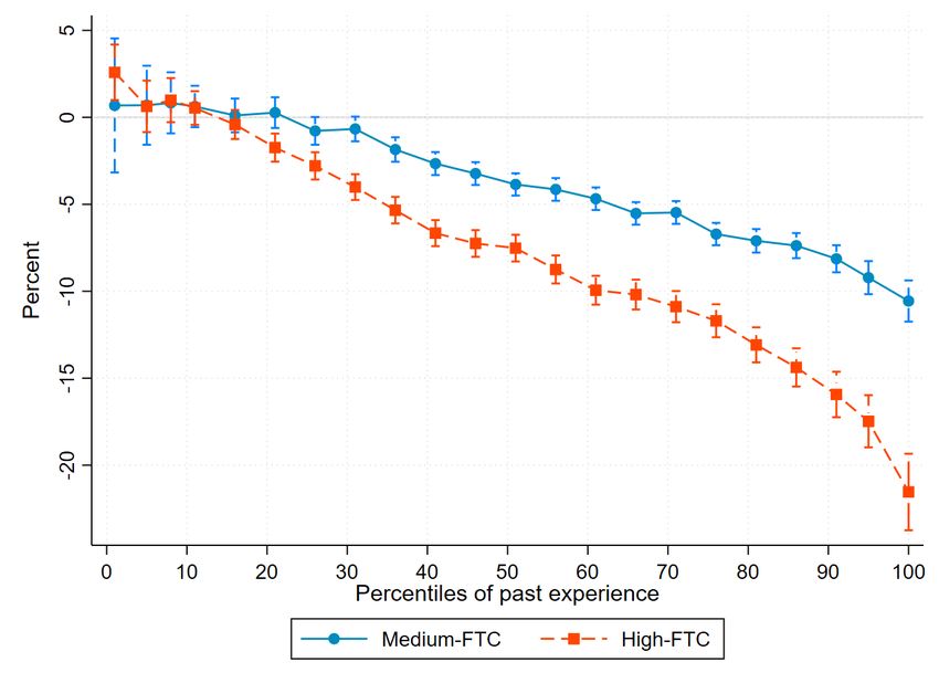
1     Introduction
Fixed-term contracts are widespread in many European countries (ter Weel, 2018). Their
extensive use is often rationalized by employers’ quest for flexibility in rigid labor markets
(Aguirregabiria and Alonso-Borrego, 2014). On the one hand, workers might benefit from
the availability of fixed-term contracts since they ease job finding (de Graaf-Zijl et al.,
2011) and mitigate wage losses associated with skill depreciation during non-employment
(Guvenen et al., 2017; Jarosch, 2021). On the other hand, temporary employment could
be detrimental if induces unstable careers (Blanchard and Landier, 2002) and lower hu-
man capital accumulation (Cabrales et al., 2017; Bratti et al., 2021). While temporary
contracts might reduce time out of work and allow workers to accumulate experience (al-
most) continuously, the quality of that experience may be worse due to poorer learning
opportunities that still translate into foregone wages.
    In this paper we shed light on how labor market duality affects human capital accu-
mulation and wage trajectories of workers during their first years in the labor market.
We perform our analysis in the context of the Spanish labor market, where the use of
fixed-term contracts is the rule rather than the exception: more than 90% of the con-
tracts signed each month are fixed-term and around 25% of the workforce is under some
form of temporary employment (Felgueroso et al., 2018). We rely on rich administrative
data that allows us to follow individuals since labor market entry and measure exact
time worked under permanent and temporary contracts, separately. We use these precise
measures of accumulated experience to estimate reduced-form wage regressions derived
from a stylized framework of human capital development in a dual labor market.
    Our results point to lower returns to past experience under fixed-term contracts rela-
tive to open-ended contracts. In particular, we find that each additional year of accumu-
lated experience in temporary employment is associated with 0.8 percentage points lower
daily wage relative to the experience accumulated in permanent jobs, after accounting for
observed match components and unobserved worker heterogeneity. Differences in returns
prevail among job switchers, suggesting a human capital channel, since for these workers
there is a clear dissociation between where experience was acquired and where it is val-
ued. However, the uncovered difference masks substantial heterogeneity among workers.
We find that the gap in returns is increasing with individual ability, being negligible for
individuals at the bottom of the ability distribution while reaching 1.6 percentage points
for high-ability workers. Similarly, while individuals with low levels of experience do not

                                              1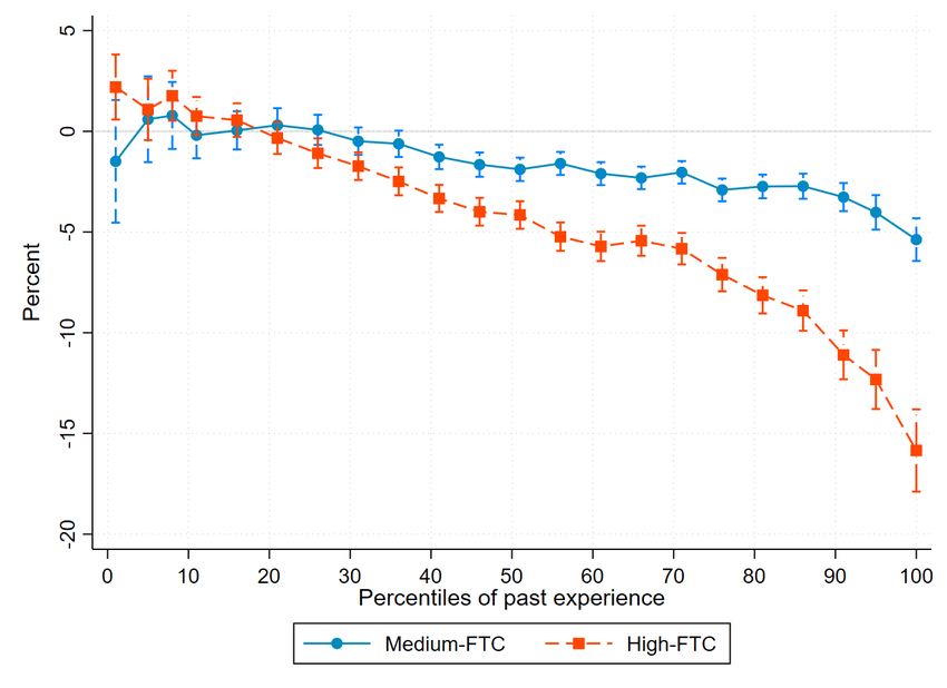
suffer losses, higher incidence of past temporary employment among highly experienced
workers leads to wage losses of up to 15%. Finally, the comparison of contract-specific
employment trajectories indicates that heterogeneous returns to experience are associ-
ated with large shifts along the distribution of wage growth after 15 years since labor
market entry.
   This paper contributes to different strands of the literature. A significant body of
research has investigated the consequences of flexibility at the margin (existence of fixed-
term contracts with low firing costs alongside highly protected open-ended contracts) for
labor market performance (Boeri, 2011; Bentolila et al., 2020). One of the dimensions
analyzed is the impact of temporary employment on workers’ careers. Although empirical
evidence on whether temporary employment is a stepping stone or a dead end to stable
employment are mixed (Filomena et al., 2021), what is less controversial is that fixed-term
contracts penalize workers in the long run, due to a less continuous employment path and
lower wage growth (Booth et al., 2002; Autor and Houseman, 2010; Garcı́a-Pérez et al.,
2019). We complement this literature by showing that even if workers are able to be
continuously working over their career, they are penalized from acquiring experience in
fixed-term contracts.
   A parallel strand of the literature has analyzed contemporaneous wage differentials
between temporary and permanent workers (e.g., Booth et al., 2002; de la Rica, 2004;
Mertens et al., 2007; Kahn, 2016; Laß and Wooden, 2019; Albanese and Gallo, 2020).
Most of the results point to a penalty for workers on fixed-term contracts, which is typi-
cally rationalized by either less firm-sponsored training (Arulampalam and Booth, 1998;
Cabrales et al., 2017; Bratti et al., 2021) or lower worker’s effort when the probability
of conversion from temporary to permanent are low (Sanchez and Toharia, 2000; Dolado
et al., 2016). Our analysis complements this literature by focusing on how past experi-
ence accrued on temporary versus permanent contracts affects current wages. Our results
suggest that the costs of being employed on temporary contracts accumulate over work-
ers’ careers, leading to lower returns to experience if on-the-job learning occurs under
fixed-term contracts.
   Finally, our analysis contributes to a growing literature that investigates the existence
of heterogeneous returns to experience due to differences in learning opportunities based
on firm type (Pesola, 2011; Arellano-Bover and Saltiel, 2021), coworkers quality (Jarosch
et al., 2021), or city size (de la Roca and Puga, 2017). We add to this line of work by

                                             2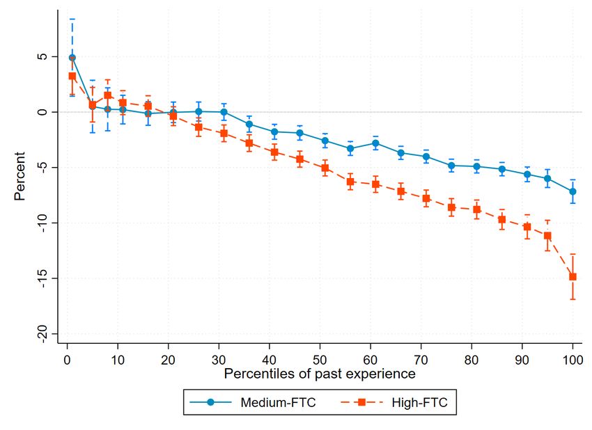
showing that skill acquisition under alternative contractual arrangements also leads to
heterogeneous wage-experience profiles.
        The remainder of the paper proceeds as follows. Section 2 presents the conceptual
framework behind our reduced-form analysis, while Section 3 describes the data. Section
4 introduces our econometric approach and discusses the results. Section 5 concludes.

2         Earnings Trajectories in a Dual Labor Market
In this section we lay out a parsimonious framework linking labor market duality to on-
the-job human capital accumulation and wage growth, which we use to derive our main
earnings equation.

Human Capital. Consider an individual i in period t. We define the stock of human
capital for this individual as
                                            Hit = ηi + hit                                           (1)

where ηi is the human capital developed before labor market entry (education level but
also innate ability) and assumed to be fixed over time while hit is the stock of human
capital accumulated since labor market entry up period t.
        Human capital, hit , is acquired on the job and varies according to the type of contract
worker i is employed in at time t. Formally, skill acquisition between two consecutive
periods is governed by the following low of motion

                                           hit+1 = hit + µcit                                        (2)

where c denotes the type of contract, fixed-term vs open-ended, and µcit is an i.i.d. draw
from contract-specific distribution F c , such that E[µcit ] = γ c . Differences in human capital
accumulation between workers with fixed-term and open-ended contracts are governed
by differences in the distributions of F c . For example, companies may be less willing
to invest in people employed on temporary contracts due to the potential finite nature
of the labor relationship (Crawford, 1988; Poulissen et al., 2021), which translates into
worse skill acquisition for workers during temporary employment episodes.1 Workers
on fixed-term contracts may also be less willing to make an effort to learn on the job
    1
    Ferreira et al. (2018) show that although workers on temporary contracts are less likely to receive
formal training, they participate more actively in informal learning than their peers in permanent con-
tracts. This higher commitment to informal training is especially acute at the beginning of their careers
to secure a permanent contract.

                                                   3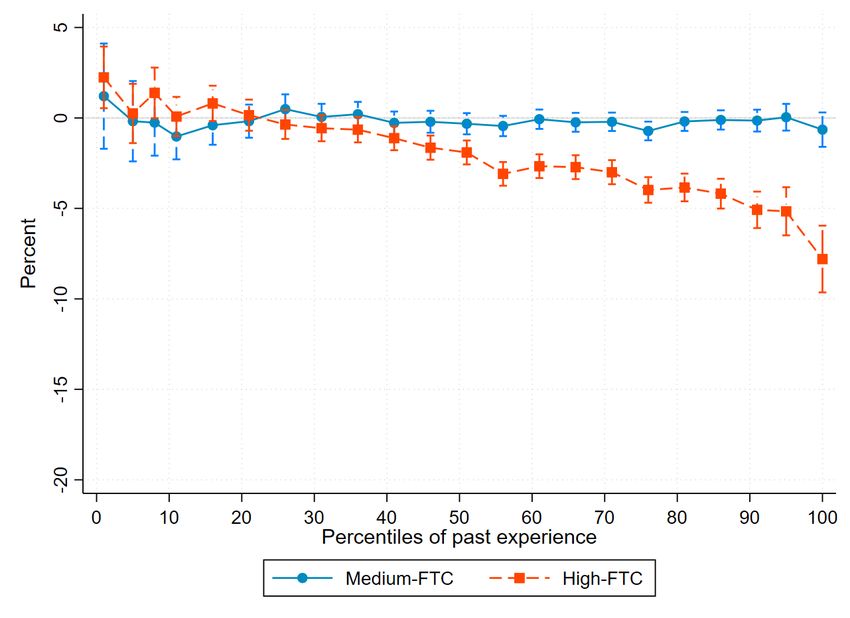
if the likelihood of contract conversion is low (Dolado et al., 2016). In the absence of
differences in skill acquisition among workers employed under different type of contracts,
human capital accumulation would depend exclusively on the total experience acquired
on the job.
      In our stylized framework the current stock of human capital accumulated since labor
market entry depends on the employment history across different contracts:
                                                         t−1
                                                         X      c(i,k)
                                                 hit =         µik                                   (3)
                                                         k=1

and
                                                    t−1
                                                    X          X
                         E[hit |oecit , ftcit ] =                        1[c(i, k) = m]γ m           (4)
                                                    k=1 m∈{ftc,oec}

where oecit and ftcit are the complete histories in open-ended and fixed-term contracts
since labor market entry up until time t, while 1[c(i, k) = m] is an indicator function
equal to one if worker i was employed under a fixed-term (ftc) or open-ended contact
(oec) in period k.2

Earnings. The structure of (log) earnings of worker i at period t is governed by the
following process
                                           ln wit = ηi + hit + Xit Ω                                 (5)

where ηi is the individual specific component, hit stands for the stock of human capital
acquired up to time t, and Xit reflects the contemporaneous job characteristics. Thus,
the expected earnings are given by

                  E[ln wit |i, Xit , oecit , ftcit ] = ηi + γ oec oecit + γ ftc ftcit + Xit Ω        (6)

where oecit and ftcit are measures of accumulated experience under open-ended and fixed-
term contracts since labor market entry up until time t, defined respectively as
                        t−1
                        X                                                   t−1
                                                                            X
              ftcit =         1[cc(i,k) = ftc]      and         oecit =           1[cc(i,k) = oec]
                        k=1                                                 k=1

      The sum of oecit and ftcit represents the standard experience component in a Mincer
regression (Mincer, 1974), which does not differentiate returns across contracts.
  2
     Individuals may have more than one job at any given time. In our empirical analysis, we count
all days worked under a given type of contract each year independently of whether is with the same
employer or under multiple ones.

                                                          4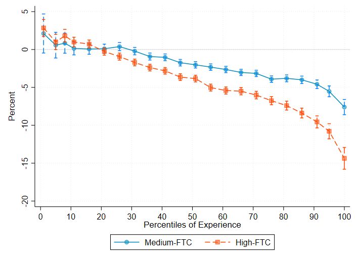
Empirical Hypothesis. In this framework, we test two hypotheses relating wage tra-
jectories in a dual labor market. Wage trajectories over the life cycle depend on human
capital accumulation, which is affected by on-the-job learning opportunities and employ-
ers’ investment in skills. To the extent the latter are higher in open-ended contracts, we
should observe a larger return to experience accumulated in this type of contract. The
first hypothesis makes this claim:

        Hypothesis 1: Human capital accumulates faster under open-ended contracts.

        Wage profiles are heterogeneous across workers and steeper for highly educated or
more skilled individuals (Heckman et al., 2006). To the extent these workers either learn
faster on the job or receive more training, we should observe a larger penalties from
accumulating experience in temporary contracts for high-ability workers. The second
hypothesis is as follows:

        Hypothesis 2: The gap in returns increases with individual ability.

        Ultimately, it is an empirical question whether we find any difference in the returns to
experience accumulated in permanent and temporary contracts. This is what we explore
in the remainder of the paper.

3         Data
Our main data source is the Spanish Continuous Sample of Employment Histories (Mues-
tra Continua de Vidas Laborales or MCVL), an administrative dataset collected annually
by the Spanish Social Security administration and linked to the Residents’ Registry and
Tax Records since 2005 up to 2018.3 The MCVL is a representative 4 percent random
sample of individuals who had any relationship with the Social Security at any time in
the reference year.4 The dataset has a longitudinal design, since an individual present in
a year and subsequently remains registered with the Social Security administration stays
    3
    The first version of the MCVL corresponds to 2004. This wave is discarded as most of the information
structure differs from that available for subsequent years.
    4
    This includes employed and self-employed workers, recipients of unemployment benefits and pension
earners, but excludes individuals registered only as medical care recipients, or those with a different
social assistance system (civil servants, such as the armed forces or the judicial power).

                                                   5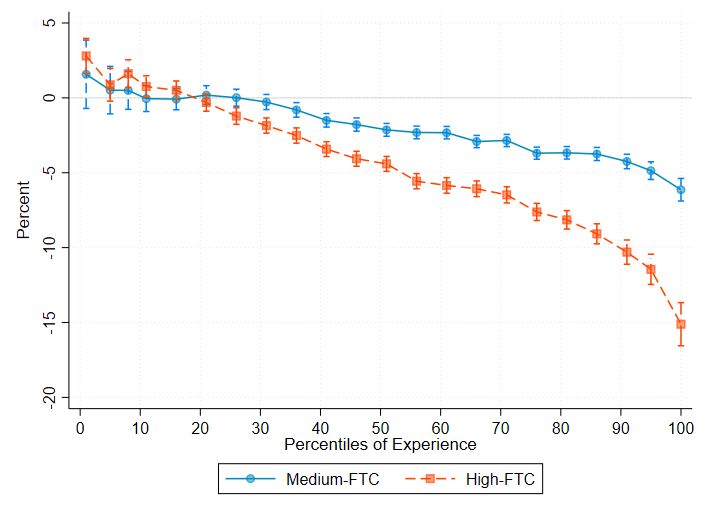
as a sample member.5 The MCVL is refreshed each year, remaining representative of
both the stock and flows of individuals.
       For each sample member, the MCVL retrieves all relationships with the Social Secu-
rity since the date of the first job spell, or 1967 for earlier entrants. All job spells are
followed from their start up to their end or to the 31st of the December of 2018. This
unique feature allows us to track individuals over time and calculate the exact number of
days worked since labor market entry. For each employment episode, we observe detailed
information on the labor relationship including part-time status, occupation category,
workplace location and sector of activity, type of contract (with reliable information
since 1997), and labor income.6 Demographic information is also reported, e.g. age,
gender, education, nationality.7
       We use the 2005-2018 MCVL original files to identify potential individuals for our
estimation sample. We exclude individuals with missing key information and focus on
those who entered the labor market after 1996 to be able to track days worked under
alternative job contracts. We exclude from the sample all foreigners because we do not
have information on any previous work experience abroad, so we cannot compute their
complete labor market history. Similarly, we remove individuals whose first employment
observations is more than 5 years after predicted graduation year, i.e. labor market entry.
We further restrict the sample to employees in the General Regime of the Social Security,
thereby excluding employment episodes in special regimes such as agriculture, fishing,
mining, or household activities as well as of self-employment. From this sample of job
spells, we construct an individual-year panel to study individual wages up to the first 15
years after predicted graduation.8 These restrictions yield a final sample of 242,774 indi-
viduals observed over a total of 1,954,097 employment (work-year) observations between
1997 and 2018. Table A.1 in the Appendix reports descriptive statistics.
   5
    Individuals who stop working remain in the sample while they receive unemployment benefits or
other welfare benefits (e.g. retirement pension). Individuals leave the sample when they die or leave the
country permanently. Likewise, each wave adds individuals who enter the labor market for the first time.
   6
    Labor income comes from Social Security contribution bases that are top-coded. We correct the
upper tail of the wage distribution by fitting cell-by-cell Tobit models to log daily wages. Appendix B
provides a detailed discussion on the correction method and offers a comparison between original and
corrected wage distributions.
   7
       Appendix C provides a detailed description of the variables.
   8
    If an individual has more than one labor relationship with different employers, we keep only the
main employer defined as the one reporting the highest annual earnings. Similarly, if an individual hold
more than one contract with the same employer within a year, we select the job characteristics coming
from the last job contract observed in that year.

                                                     6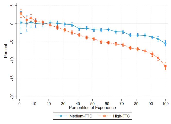
4        Returns to Experience in a Dual Labor Market
4.1       Econometric Model
Returns to Experience. The stylized framework in Section 2 provides us with a flex-
ible specification to estimate the returns to experience under different type of contracts.
To this purpose we adapt equation (6) and estimate a linear panel data model for the
logarithm of real daily wages of individual i and year t
                                    X
                     ln wit = ηi +        γ c cit + Xit Ω + δe + δt + it                                 (7)
                                            c∈{ftc,oec}

       where ηi stands for pre-labor market permanent individual ability while oecit and ftcit
measure the experience accumulated by worker i working under open-ended or fixed-term
contracts respectively, since labor market entry up to time t.9 Xit refers to contempora-
neous job-firm characteristics (tenure, type of contract, part-time status, skill level, plant
size and age, location, and sector of activity), whereas δe and δt are potential experience
and year fixed effects, respectively.10 The inclusion of potential experience effects along
with contemporaneous job-firm characteristics ensures that differences in the returns to
accumulated experience can only be driven by heterogeneous past histories in the labor
market. Individual fixed effects are intended to account for the sorting of workers based
on unobserved permanent heterogeneity. Under the assumption that it is an i.i.d. ran-
dom term, consistent estimates can be obtained by applying the standard panel fixed
effects estimator.11

Unobserved Learning Abilities. To explore complementarities between individual
ability and experience acquired in different contracts, we introduce worker heterogeneity
in the form of unobserved ability to learn. More specifically, we incorporate the interaction
between ability and the learning benefits of fixed-term and open-ended contracts into our
framework and extend equation (7) as follows
                        X                X
          ln wit = ηi +        γ c cit +                           ϕc ηi cit + Xit Ω + δe + δt + it      (8)
                              c∈{ftc,oec}            c∈{ftc,oec}

   9
     For simplicity, we only include experience terms linearly but we also estimate Equation (7) using a
step-wise specification for contract-specific returns to experience with 22 cut-off points.
  10
     We include potential experience fixed effects, i.e., years since entry into the labor market, rather than
age effects because some age groups are only identified by the less educated individuals. For example,
college graduates are not observed before reaching the age of 24. In addition, accounting for potential
experience effects ensures that we are comparing individuals at the same point in their careers.
  11
    For comparison we also estimate a version of this model without individual fixed effects, including
education level and a female indicator to control for pre-labor market human capital.

                                                          7
where we allow the value of experience accumulated in different contracts to vary among
individuals. The parameter ϕc captures whether higher-ability workers face larger returns
to experience acquired at different contracts. To estimate equation (8) we follow the
algorithm proposed by de la Roca and Puga (2017).12
Scarring Effects. Differences in returns to contract-specific experience could be due
to heterogeneous rates at which experience is accumulated, not just differences in skill
acquisition. Workers under temporary contracts may have more job interruptions than
individuals employed in permanent positions and non-working episodes could result into
lower experience levels (and lower human capital overall). To control for this margin, we
adapt our benchmark model and compare individuals with the same level of total experi-
ence but different incidence of temporary employment in their career. In particular, each
year, we discretize our overall experience measure into Q-bins such that q = {{0}, (0, 4],
(4, 7], (7, 10], (10, 15], ..., (95, 97], (97, 100]} and estimate the following regression model
Q
3 X
X
ln wit = ηi + βm(q) 1{expit = q} × 1{ftcit = m} + Xit Ω + δe + δt + it (9)
m=1 q=0
where 1{expit = q} takes value one if worker i falls into the qth-bin of actual experience
in period t. We then interact this variable with an indicator for the incidence of temporary
employment during the acquisition of experience. More precisely, we create three group of
workers based on the ratio of experience under fixed-term contracts to overall experience:
low (ratio lower than 0.3), medium (between 0.3 and 0.9) and high incidence (above 0.9).
Thus, 1{ftcit = m} is an indicator variable identifying workers in a given group according
to the incidence of temporary employment since labor market entry up to time t. Notice
that the parameters βm(q) are only identified up to a normalization. We impose the impact
of accumulated experience on individuals wages to be zero for the first observation, when
experience in the labor market is equal to zero. This implies that βm(0) is equal to zero
for each of the three m-groups, thereby estimating for each m-group 22 parameters. The
point estimates β2(q) and β3(q) capture the wage gap between individuals who have been
employed for the same amount of time since labor market entry but have had a higher
12
The algorithm requires to guess a set of individual fixed effects, ηi0 , estimate equation (8) by OLS,
obtain a new set of estimates of worker fixed effects as
ln wit − c∈{ftc,oec} γ c cit − Xit Ω − δe − δt
P
1
ηi = P c
c∈{ftc,oec} ϕ cit
and use them as new guess until convergence is achieved.
8incidence of temporary employment in the past. Hence equation (9) allows us to quantify
the value of experience in fixed-term contracts relative to permanent contracts, comparing
workers with the same level of experience acquired under different work histories due to
the heterogeneous incidence of temporary employment.
4.2 Results
Dual Returns to Experience. We start our discussion on how skill acquisition under
different type of contracts affect wages by looking at the returns to experience estimated
from Equation (7). To ease the interpretation, we estimate standard Mincerian returns to
experience and then differential returns by type of contract, with and without individual-
level unobserved heterogeneity. The results, displayed in Table 1 Panel A, show that
each additional year of experience raises individual wages by 2.9%, or by 4.9% if both
contemporaneous job-firm characteristics and individual heterogeneity are taken into ac-
count. However, the returns to experience vary depending on whether such experience
was accumulated under fixed-term (FTC) or open-ended (OEC) contracts. Consistent
with the first hypothesis, an additional year of experience in permanent contracts is as-
sociated with wage gains of 3.5%, while returns are 1.5 percentage points (pp) lower for
experience accumulated in temporary jobs. The difference is reduced once unobserved
individual heterogeneity is factored in (∼0.8pp), suggesting that the sorting of workers
into contractual arrangements (and other observed match components) is important, but
does not fully explain the gap in returns.13 To the extent the link between current wages
and past experience reveals past skill development of workers, our findings are consistent
with lower on-the-job learning while employed under FTC.
To strengthen our findings, we look at the first re-employment observation of workers
who switched jobs in our sample (see Table 1 Panel B). In this fashion, we can dissociate
the place where experience has been accumulated from the place where that experience
is being valued and thus shed light on the human capital channel. The results are aligned
with our baseline estimates: returns to experience acquired under OEC are higher relative
to FTC experience (∼0.6pp gap). This supports the idea of contract-specific on-the-job
learning, which implies lower accumulation of human capital during temporary employ-
13
Our results are robust to alternative measures of labor income (Table A.2) as well as different spec-
ifications to account for life-cycle differences such a cubic polynomial on potential experience, excluding
potential experience fixed-effects, or using age fixed effects (Table A.3). Heterogeneous returns to ex-
perience also arise when modelling contract-specific experience non-parametrically using step functions
with 22 cut-off points, but the gap between OEC and FTC is non-linear (Figure A.1).
9ment episodes.
Table 1: Dual Returns to Experience
A. All Workers OLS Fixed-Effects
(1) (2) (3) (4)
Experience 0.0293*** 0.0496***
(0.0003) (0.0005)
Experience OEC 0.0350*** 0.0499***
(0.0003) (0.0005)
Experience FTC 0.0209*** 0.0421***
(0.0004) (0.0006)
Observations 1,954,097 1,954,097 1,954,097 1,954,097
R-squared 0.6330 0.6343 0.3058 0.3064
B. Job Switchers OLS Fixed-Effects
(1) (2) (3) (4)
Experience 0.0303*** 0.0482***
(0.0003) (0.0006)
Experience OEC 0.0347*** 0.0492***
(0.0004) (0.0006)
Experience FTC 0.0245*** 0.0436***
(0.0004) (0.0008)
Observations 590,080 590,080 590,080 590,080
R-squared 0.6019 0.6025 0.3432 0.3433
Notes: Experience is measured in days and then it is transformed into years. OEC and
FTC stand for experience acquired under open-ended and fixed-term contracts, respec-
tively. All specifications include controls for a quadratic polynomial in tenure, type of
contract, a dummy for part-time jobs, indicators for occupation-skill category (2), sector
of activity (10), workplace location (50), small and medium enterprises (plant size < 50),
young organizations (plant age < 10), potential experience dummies (5), and year dum-
mies (22). OLS regressions include additional controls for education and gender. Standard
errors clustered at the individual level in parenthesis. Panel B specification uses only the
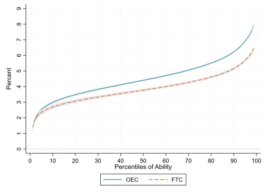
first re-employment observation after job change. Job switchers = 200,491. *** preturns to experience accumulated while working on OECs are 1.6pp higher than returns
to experience from temporary employment. Consistent with the second hypothesis, this
greater difference may be due to the fact that wage-experience profiles are steeper among
highly educated individuals, who can take full advantage of better learning opportunities
provided during open-ended jobs.
Table 2: Dual Returns to Experience: Worker’s Observables
Gender Education
Male Female Non-College College
Experience OEC 0.0506*** 0.0489*** 0.0421*** 0.0589***
(0.0006) (0.0007) (0.0005) (0.0009)
Experience FTC 0.0405*** 0.0426*** 0.0428*** 0.0436***
(0.0008) (0.0008) (0.0007) (0.0011)
Observations 934,294 1,019,803 1,180,999 773,098
R-squared 0.2870 0.3242 0.3051 0.3053
Notes: Experience is measured in days and then it is transformed into years. OEC
and FTC stand for experience acquired under open-ended and fixed-term contracts,
respectively. Non-college includes both high-school dropouts and graduates. All spec-
ifications include the same set of controls as Column (4) in Table 1. Standard errors
clustered at the individual level in parenthesis. *** pFigure 1: Dual Returns to Experience: Unobserved Ability
Notes: Contract-specific returns to experience computed for each percentile of unobserved ability us-
ing estimates (×100) from equation (8). 95% confidence bands are calculated using the clustered-wild
bootstrap (100 repetitions) procedure by Cameron et al. (2008). OEC and FTC stand for experience
acquired under open-ended and fixed-term contracts, respectively.
additional year of OEC (FTC) experience translates into 8% (6.4%) higher earnings.14
Scarring Effects. While temporary employment seems to generate a gap in returns
through lower skill acquisition, it could also reduce overall actual experience because
of job interruptions and induce skill depreciation. Hence, to shed light on the scarring
effects of temporary employment on wages due to less on-the-job learning, we compare
workers who have the same actual experience but accumulated differently due to the
heterogeneous incidence of temporary contracts since labor market entry up to time t.
Figure 2 plots β2(q) and β3(q) parameters from equation (9), which can be interpreted
as the scarring effects of temporary employment, as they proxy by means of current
wages the human capital investment foregone during the acquisition of experience during
temporary employment episodes. The estimates reveal several interesting patters. First,
we do not find a negative impact of higher incidence of temporary employment among
14
We have also experimented with a quantile regression approach to estimate the equation 7. The
results are consistent with the existence of heterogeneous returns across the skill distribution: difference
in returns widens along the wage distribution. Results are available upon request.
12Figure 2: Scarring Effects of Temporary Employment
Notes: Estimates (×100) and 95% confidence intervals of the scarring effects of temporary employment,
β2(q) and β3(q) , from equation (9). Standard errors are clustered at the individual level. Medium-FTC
(High-FTC) incidence refers to individuals whose actual experience on a temporary contract relative to
overall actual experience is between 0.3 and 0.9 (above 0.9).
low experienced individuals. Second, wage losses become apparent from the fortieth per-
centile of overall experience onward. distribution. Third, the greater the acquisition
of experience through fixed-term contracts, the greater the losses. Finally, highly ex-
perienced individuals face wage losses of up to 15% due to higher incidence of FTC in
the past. These findings are indicative of poorer learning opportunities face by workers
during temporary employment episodes which translates into lower earnings.
Counterfactual Wage Trajectories. Finally, we assess how much dual learning on-
the-job can affect earnings trajectories. We do this by comparing wage growth 15 years
after labor market entry for alternative labor market histories based on the incidence of
the two contractual arrangements. Specifically, we use estimates from equation (8) to
predict counterfactual wage growth for workers who spent 15 years in OEC and compare
it to the alternative scenario when the worker experienced 15 years in FTC. Given the
complementarity between ability and returns to experience, we look at low and high
ability workers under the two scenarios described above. To put these values in context,
13Table 3: Life-Cycle Wage Trajectories
Counterfactual Actual
Wage Growth, Wage Growth,
Unobserved Ability Employment Trajectory % Percentiles
10th Percentile Always in FTC 37.75 40
10th Percentile Always in OEC 41.86 43
90th Percentile Always in FTC 72.21 62
90th Percentile Always in OEC 87.15 73
Notes: Wage growth calculated as the log difference between entry-level daily wages and daily
wages observed 15 years after. Counterfactual wage growth is computed for alternative employment
trajectories based on the continuous incidence of OEC or FTC and using (unobserved) ability-
specific returns from equation 8. Actual wage growth stands for wage growth for workers observed
during 15 years in the labor market.
we compare them to the wage growth observed after 15 years of potential experience and
report the associated percentile in the distribution.15
Table 3 reports the results of this exercise. On the one hand, low-skill workers do
not suffer any significant penalty from accumulating experience in FTC. After 15 years
since entering the labor market, workers who have always been employed in OEC would
face 5pp higher wage growth, allowing them to move only marginally in the wage growth
distribution (from the 40th to the 43rd percentile). On the other hand, high-skill workers
would significantly suffer from accumulating experience only through FTC. In particular,
we find that the wage penalty of being continuously employed under FTC relative to OEC
amounts to roughly 15pp, corresponding to a shift from the 73rd to the 62nd percentile
of the wage growth distribution.
5 Conclusions
In this paper we document how labor market duality affects human capital accumulation
and life-cycle wage profiles of young workers. We implement our analysis in the context
of the Spanish labor market, which is characterized by a strong segmentation between
fixed-term and open-ended contracts.
Our results point to lower returns to experience acquired while working under fixed-
term contracts compared to permanent jobs, suggesting less on-the-job learning during
temporary employment episodes. However, the gap in returns shows significant hetero-
15
To compute the actual wage growth distribution, we rely only on the oldest cohorts for whom we
observed 15 years of potential experience.
14geneity among workers. We show that differences increase as a function of individual
ability, suggesting a strong complementarity between contract-related learning opportu-
nities and individual ability. We also document substantial wage losses among workers
with the same experience who faced a higher incidence of temporary employment in the
past, which we take as evidence of foregone income due to lower skill acquisition under
fixed-term contracts.
Taken together, our findings suggest numerous policy considerations. Heterogeneous
returns across contracts bear implications for life-cycle wage inequality, hence policy tar-
geted at increasing human capital accumulation in temporary contracts (e.g. on-the-job
training subsidies) could be beneficial in reducing long-run wage differences. Moreover,
our results hint that the negative impact of labor market duality on workers’ early careers
extends beyond unstable work histories, as experience accumulated while employed under
fixed-term contracts is less valuable. While the joint evaluation of both margins along
with employer’s training choices would require the use of a more structural model, we
leave that for future research.
References
Aguirregabiria, V. and Alonso-Borrego, C. (2014). Labor Contracts and Flexibility: Ev-
idence from a Labor Market Reform in Spain. Economic Inquiry, 52(2):930–957.
Albanese, A. and Gallo, G. (2020). Buy flexible, Pay More: The Role of Temporary
Contracts on Wage Inequality. Labour Economics, 64:101814.
Arellano-Bover, J. and Saltiel, F. (2021). Differences in On-the-Job Learning Across
Firms. IZA DP No. 14473.
Arulampalam, W. and Booth, A. L. (1998). Training and Labour Market Flexibility: Is
There a Trade-off? British Journal of Industrial Relations, 36(4):521–536.
Autor, D. H. and Houseman, S. N. (2010). Do Temporary-Help Jobs Improve Labor
Market Outcomes for Low-Skilled Workers? Evidence from ”Work First”. American
Economic Journal: Applied Economics, 2(3):96–128.
Bentolila, S., J., D. J., and F., J. J. (2020). Dual Labor Markets Revisited. Oxford
Research Encyclopedia of Economics and Finance.
15Blanchard, O. and Landier, A. (2002). The Perverse Effects of Partial Labour Market
Reform: Fixed-Term Contracts in France. The Economic Journal, 112(480):F214–
F244.
Boeri, T. (2011). Institutional Reforms and Dualism in European Labor Markets. In
Card, D. and Ashenfelter, O., editors, Handbook of Labor Economics, volume 4, pages
1173–1236. Elsevier, Amsterdam: North-Holand.
Bonhomme, S. and Hospido, L. (2017). The Cycle of Earnings Inequality: Evidence from
Spanish Social Security data. The Economic Journal, 127(603):1244–1278.
Booth, A. L., Francesconi, M., and Frank, J. (2002). Temporary Jobs: Stepping Stones
or Dead Ends? The Economic Journal, 112(480):F189–F213.
Bratti, M., Conti, M., and Sulis, G. (2021). Employment Protection and Firm-Provided
Training in Dual Labour Markets. Labour Economics, 69:101972.
Cabrales, A., Dolado, J. J., and Mora, R. (2017). Dual Employment Protection and (lack
of) On-the-Job Training: PIAAC Evidence for Spain and Other European Countries.
SERIEs, 8(4):345–371.
Cameron, A. C., Gelbach, J. B., and Miller, D. L. (2008). Bootstrap-Based Improvements
for Inference with Clustered Errors. The Review of Economics and Statistics, 90(3):414–
427.
Card, D., Heining, J., and Kline, P. (2013). Workplace Heterogeneity and the Rise of
West German Wage Inequality. Quarterly Journal of Economics, 128(3):967–1015.
Crawford, V. P. (1988). Long-Term Relationships Governed by Short-Term Contracts.
The American Economic Review, 78(3):485–499.
de Graaf-Zijl, M., Van den Berg, G. J., and Heyma, A. (2011). Stepping Stones for the
Unemployed: The Effect of Temporary Jobs on the Duration until (Regular) Work.
Journal of Population Economics, 24(1):107–139.
de la Rica, S. (2004). Wage Gaps Between Workers with Indefinite and Fixed-term
Contracts: The Impact of Firm and Occupational Segregation. Moneda y Credito,
219(1):43–69.
16de la Roca, J. and Puga, D. (2017). Learning by Working in Big Cities. The Review of
Economic Studies, 84(1):106–142.
Dolado, J. J., Ortigueira, S., and Stucchi, R. (2016). Does Dual Employment Protection
Affect TFP? Evidence from Spanish Manufacturing Firms. SERIEs, 7(4):421–459.
Dustmann, C., Ludsteck, J., and Schoenberg, U. (2009). Revisiting the German Wage
Structure. Quarterly Journal of Economics, 124(2):843–881.
Felgueroso, F., Garcı́a-Pérez, J. I., Jansen, M., and Troncoso-Ponce, D. (2018). The
Surge in Short-Duration Contracts in Spain. De Economist, 166(4):503–534.
Ferreira, M., de Grip, A., and van der Velden, R. (2018). Does Informal Learning at
Work Differ Between Temporary and Permanent Workers? Evidence from 20 OECD
Countries. Labour Economics, 55:18–40.
Filomena, M., Picchio, M., et al. (2021). Are Temporary Jobs Stepping Stones or Dead
Ends? A Meta-Analytical Review of the Literature. IZA DP No. 14367.
Garcı́a-Pérez, J. I., Marinescu, I., and Vall Castello, J. (2019). Can Fixed-term Contracts
Put Low Skilled Youth on a Better Career Path? Evidence from Spain. The Economic
Journal, 129(620):1693–1730.
Guvenen, F., Karahan, F., Ozkan, S., and Song, J. (2017). Heterogeneous Scarring Effects
of Full-Year Nonemployment. American Economic Review, 107(5):369–73.
Heckman, J. J., Lochner, L. J., and Todd, P. E. (2006). Earnings Functions, Rates of
Return and Treatment Effects: The Mincer Equation and Beyond. volume 1, pages
307–458. Elsevier, Amsterdam: North-Holand.
Jarosch, G. (2021). Searching for Job Security and the Consequences of Job Loss. NBER
WP No.28481.
Jarosch, G., Oberfield, E., and Rossi-Hansberg, E. (2021). Learning From Coworkers.
Econometrica, 89(2):647–676.
Kahn, L. M. (2016). The Structure of the Permanent Job Wage Premium: Evidence from
Europe. Industrial Relations: A Journal of Economy and Society, 55(1):149–178.
17Laß, I. and Wooden, M. (2019). The Structure of the Wage Gap for Temporary Work-
ers: Evidence from Australian Panel Data. British Journal of Industrial Relations,
57(3):453–478.
Mertens, A., Gash, V., and McGinnity, F. (2007). The Cost of Flexibility at the Margin.
Comparing the Wage Penalty for Fixed-term Contracts in Germany and Spain using
Quantile Regression. LABOUR, 21(4-5):637–666.
Mincer, J. (1974). Schooling, Experience, and Earnings. . Human Behavior & Social
Institutions No. 2.
Pesola, H. (2011). Labour Mobility and Returns to Experience in Foreign Firms. The
Scandinavian Journal of Economics, 113(3):637–664.
Poulissen, D., De Grip, A., Fouarge, D., and Künn-Nelen, A. (2021). Employers’ Willing-
ness to Invest in the Training of Temporary Workers: A Discrete Choice Experiment.
IZA DP No. 14395.
Sanchez, R. and Toharia, L. (2000). Temporary Workers and Productivity: The Case of
Spain. Applied Economics, 32(5):583–591.
ter Weel, B. (2018). The Rise of Temporary Work in Europe. De Economist, 166(4):397–
401.
18A Supplementary Tables and Figures
Table A.1: Descriptive Statistics
Mean Std. Dev
Female 0.523 -
College 0.396 -
Age at Entry 22.30 3.16
Wage at Entry 39.51 22.59
Days Worked at Entry 189.56 105.18
under OEC 33.71 85.48
under FTC 155.85 106.45
Years in the Labor Market 10.50 4.53
Experience (yrs) 5.82 4.49
under OEC 3.22 3.87
under FTC 2.60 2.56
Annual Wage Growth 0.065 0.172
Workers 242,774
Worker-Year Obs. 1,954,097
Notes: Entry refers to the first year of employment after the
predicted year of graduation. Accumulated experience refers to
the last individual observation. Years in the labor market refers
to the average amount of time we observe workers employed
in our sample. Experience is measured using daily information
and transformed into years. Annual wage growth corresponds to
year-on-year wage growth averaged over all observations. Wages
are in 2018 euros.
Table A.2: Robustness to Income Measure: Returns to Experience Accumulated under
Different Contracts
Censored Tax Data Pooled Income
Experience OEC 0.0398*** 0.0474*** 0.0495***
(0.0004) (0.0006) (0.0005)
Experience FTC 0.0370*** 0.0410*** 0.0439***
(0.0006) (0.0007) (0.0006)
Observations 1,954,097 1,508,948 1,954,097
R-squared 0.3112 0.2306 0.2685
Notes: Experience is measured in days and then it is transformed into years.
OEC and FTC stand for experience acquired under open-ended and fixed-term
contracts, respectively. Censored specification uses original labor income with-
out correcting for top-coding. Tax data uses information on income coming
from tax records for the period 2005-2018. Pooled income consider as measure
of daily wages income earned from all employers in a given year divided by total
days worked in such year. All specifications control for the same variables as
the fixed effect panel data model estimates in Column (4) in Table 1. Standard
errors clustered at the individual level in parenthesis. *** pTable A.3: Robustness to Life-Cycle Control: Returns to Experience Accumulated
under Different Contracts
Cubic Potential Exp. Excl. Potential Exp Age Effects
(1) (2) (3)
Experience OEC 0.0513*** 0.0456*** 0.0481***
(0.0005) (0.0005) (0.0005)
Experience FTC 0.0432*** 0.0393*** 0.0414***
(0.0006) (0.0006) (0.0006)
Observations 1,954,097 1,954,097 1,954,097
R-squared 0.3152 0.3080 0.3089
Notes: Experience is measured in days and then it is transformed into years. OEC and FTC
stand for experience acquired under open-ended and fixed-term contracts, respectively. Potential
experience stands for number of years after labor market entry. All specifications control for the
same variables as the fixed effect panel data model estimates in Column (4) in Table 1 except
for potential experience fixed effects. Column (1) controls parametrically for potential experience
but includes only the squared and cubic terms of potential experience, as the linear term is not
identified in the presence of year and individual fixed effects. Column (2) does not include any
control for life-cycle differences. Column (3) includes as control fixed effects for age-categories.
Standard errors clustered at the individual level in parenthesis. *** pFigure A.2: Robustness to Thresholds: Scarring Effects of Temporary Employment
(a) (b)
Notes: Estimates (×100) and 95% confidence intervals of the scarring effects of temporary employment,
β2(q) and β3(q) , from equation 9. Standard errors are clustered at the individual level. Medium-FTC
(High-FTC) incidence refers to individuals whose actual experience on a temporary contract relative to
overall actual experience is in Panel (a) between 0.5 and 0.9 (above 0.9) and in Panel (b) between 0.3
and 0.6 (above 0.6).
Figure A.3: Scarring Effects of Temporary Employment by Gender
(a) Men (b) Women
Notes: Estimates (×100) and 95% confidence intervals of the scarring effects of temporary employment,
β2(q) and β3(q) , from equation 9 estimated separately by gender. Standard errors are clustered at the
individual level. Medium-FTC (High-FTC) incidence refers to individuals whose actual experience on a
temporary contract relative to overall actual experience is between 0.3 and 0.9 (above 0.9).
21Figure A.4: Scarring Effects of Temporary Employment by Education Level
(a) Non-College (b) College
Notes: Estimates (×100) and 95% confidence intervals of the scarring effects of temporary employment,
β2(q) and β3(q) , from equation 9 estimated separately by education level. Standard errors are clustered at
the individual level. Medium-FTC (High-FTC) incidence refers to individuals whose actual experience
on a temporary contract relative to overall actual experience is between 0.3 and 0.9 (above 0.9).
22B Censoring Correction
The MCVL reports data on monthly labor income from Social Security contribution,
which are either bottom or top-coded. In the data, around 13 percent of the log real
daily wages of the worker-month observations are top-coded.16
Following other studies that face censored earnings in administrative data (Dustmann
et al., 2009; Card et al., 2013; Bonhomme and Hospido, 2017), we correct the upper tail by
fitting cell-by-cell Tobit models to log real daily wages separately by gender. Each cell, c,
is defined according to occupational groups (3 categories), age groups (5 categories), and
years (39) for a total of 2×450 cells. Consistent with a vast literature that finds that log-
normality provides a reasonable approximation to empirical wage distributions, within
each cell, log-daily wages are assumed to follow a Gaussian distribution with cell-specific
mean and variance, i.e. log w ∼ N (Xβc , σc2 ).17
The parameters of interest are estimated within each cell by maximum likelihood.
Denoting Φ the standard normal cdf, the cell-specific maximum likelihood takes the
following form (up to an additive constant).
h i
ln(w̄)−Xijt βc
− 21 ln σc2 1 2
P P
censit =0 − 2σc2
(ln(wijt ) − Xit βc ) + censijt =1 ln 1 − Φ σc
where wit represents real log daily wages of individual i in plant j in moment t (a worker-
month pair), w̄ is the maximum cap, censijt = 1 if the observation is top-coded. Xijt is a
set of controls such as age, categorical variables for full-time jobs, sector of activity (10),
workplace location (50), firm age (3), and monthly dummies (12). Following Card et al.
(2013), we also include individual-specific components of the wages using the mean log
daily wages in other months, fraction of censored wages in other months, and a dummy
for individuals observed only once as additional controls. For individuals who are only
observed once, we set the mean log daily wages to the sample mean, and the fraction of
censored wages to the share of censored earnings in the sample.
After the estimation, we impute an uncensored value for each censored observation
16
Less than 8 percent of the observations are bottom-coded. However, we do not correct the lower tail
due to the existence of a national minimum wage.
17
The choice of the distribution is important and a natural concern is that the results may differ
depending on the technique. In this sense, Dustmann et al. (2009) offer an extensive robustness analysis
in which they evaluate four different distributional assumptions, and conclude that the results are similar
to different specifications. Similarly, Bonhomme and Hospido (2017) use the MCVL to compare the
performance of the cell-by-cell Tobit model and a linear quantile censoring correction method with
respect to non-censored earnings coming from tax records, and find that the fit is superior with the
Tobit model.
23using the maximum likelihood estimates of each Tobit model. Specifically, we replace
censored observation by the sum of the predicted wages and a random component, drawn
from a normal distribution with mean zero and cell-specific variance. The imputation
rule is:
h i
ln w̄−Xijt β̂c ln w̄−Xijt β̂c
lnwijt = Xijt β̂c + σ̂c Φ−1 Φ σ̂c
+ u ijt × 1 − Φ σ̂c
where (β̂c , σ̂c ) are the maximum likelihood estimates of each cell, Φ denotes the standard
normal cdf, and u represents a random draw from the uniform distribution, U [0, 1].
Table C.1: Censored and imputed wage distributions
Percentiles Censored Imputed
5th 3.00 3.00
10th 3.33 3.33
25th 3.70 3.70
50th 4.04 4.04
75th 4.43 4.45
90th 4.74 5.17
95th 4.78 5.68
Notes: Wages refer to log real daily wages
earned by workers in a given employer each
month. Moments of the the log daily wage dis-
tribution are computed over month-worker-firm
observations (93,407,145).
24C Variables Definition
Birth date. Obtained from personal files coming from the Spanish Residents registry.
We select this information from the most recent wave and, if there is any inconsistency,
we choose the most common value over the waves for which it is available.
Education. Retrieved from the Spanish Residents registry up to 2009, and from 2009
thereafter the Ministry of Education directly reports individuals’ educational attainment
to the National Statistical Office and this information is used to update the corresponding
records in the Residence registry. Therefore, the educational attainment is imputed
backwards whenever it is possible, i.e. when a worker is observed in the MCVL post-
2009. In the imputation, we assigned 25 years as the minimum age to recover values
related to university education.18
Gender. Obtained from the Spanish Residence registry. We select this information
from the most recent wave and, if there is any inconsistency, we choose the mode over
the waves in which it is available.
Nationality. Obtained from Spanish Residents registry. The variable reports the link
between the individual and Spain in terms of legal rights and duties. This variable
allows to distinguish between individuals with Spanish nationality (N00 code) and other
worldwide nationalities.
Labor market entry. To define labor market entry, we exploit information on educa-
tion attainment and compute predicted graduation year of each individual. Specifically,
education-specific graduation years are assigned as the years when high-school drop-outs
turn 16, people with high-school degrees turn 18, and college graduates turn 23. We track
workers after their predicted graduation year to compute time employed and out-of-work.
Experience. Defined as the time actually worked relative to overall time after labor
market entry. We compute actual working days using information on all the spells avail-
able for each worker in the MCVL since labor market entry. Specifically, at each year t,
we count the exact number of days worked and compute our measure of experience as the
18
The age threshold is the average graduation age for a Bachelor’s degree in Spain: https://www.
oecd.org/education/education-at-a-glance-19991487.htm
25share of time actually worked in the past relative to the potential time that an individual
could have worked since labor market entry.
Labor income. The MCVL reports labor income from two different sources: Social
Security contribution basis and income tax records. Contribution bases capture gross
monthly labor earnings plus one-twelfth of year bonuses.19 Earnings are bottom and top-
coded. The minimum and maximum caps vary by Social Security regime and contribution
group, and they are adjusted each year according to the evolution of the minimum wage
and inflation rate. The data is supplemented with information provided by the Fiscal
Authorities on the total wages that employers pay to employees on an annual basis.
The advantage of this measure is that it is not censored. However, fiscal information
is only included from 2005 onwards and excludes Basque Country and Navarra. Our
main analysis relies on labor income coming from Social Security contributions and we
correct top-censored earnings fitting cell-by-cell Tobit models to log real daily wages (see
Appendix B).
Employment status. An individual is considered to be employed in a given year if
annual income is at least equal to one quarter of full-time work at half of the minimum
wage.
Contract type. The MCVL contains a long list of contract types (over 100) that
are summarized in two broad categories, according to its permanent or temporary na-
ture. Permanent contracts include regular permanent contracts (contrato indefinido fijo)
and intermittent (seasonal) permanent contracts (indefinido fijo-discontinuo). Tempo-
rary contracts include specific project or service contracts (temporal por obra o servicio),
temporary increase in workload (eventual de produccion), and substitution contracts (in-
terinidad o relevo).
Occupation category. Based on Social Security contribution group. These groups in-
dicate a level in a ranking determined by the worker’s contribution to the Social Security
system, which is determined by both the education level required for the specific job and
the complexity of the task. The MCVL contains 10 different contribution groups that are
aggregated according to similarities in skill requirements. High-Skill: Group 1 (engineers,
19
Exceptions include extra hours, travel and other expenses, and death or dismissal compensations.
26college, senior managers —in Spanish ingenieros, licenciados y alta direccion), Group 2
(technicians —ingenieros tecnicos, peritos y ayudantes), and Group 3 (administrative
managers —jefes administrativos y de taller ). Medium-Skill: Group 4 (assistants —ayu-
dantes no titulados) and Group 5-7 (administrative workers —oficiales administrativos
(5), subalternos (6) and auxiliares administrativos (7)). Low-Skill: Group 8-10: (manual
workers —oficiales de primera y segunda (8), oficiales de tercera y especialistas (9) y
mayores de 18 años no cualificados (10)).
Establishment. Defined by its Social Security contribution account (codigo de cuenta
de cotizacion). Each firm is mandated to have as many accounts as regimes, provinces,
and relation types with which it operates. The contribution accounts are assigned by the
Social Security administration, and they are fixed and unique for each treble province-
Social Security regime-type of employment relation.20 Thus, contribution accounts can
be thought of as establishments.
Establishment creation date. Date when the first employee was registered in the
contribution account. We rely on this date as a proxy for the workplace creation date to
classify employers into age bins.
Establishment size. Number of employees working in the establishment at the mo-
ment of data extraction. Unfortunately, this variable is missing before 2005. For the
years in which the variable is missing, we assigned the average size observed for that
establishment from 2005 onwards. In the case of establishments not observed after 2005,
we assigned a value of zero.21
Establishment location. The municipality in which the establishment conducts its
activity if above 40,000 inhabitants, or the province for smaller municipalities (domicilio
de actividad de la cuenta de cotizacion). Based on that, we group all locations into the
50 Spanish provinces.
20
According to the Social Security administration, around 85 percent of the firms are single unit
organizations, i.e. there have just one contribution account per firm. Each firm has typically one
account for each treble province-Social Security regime-type of employment relation.
21
We tested our results by including a dummy variable in our regressions to identify firms not observed
after 2004. However, our main results are not affected, so we avoid including such an indicator.
27Sector of activity. The MCVL provides information on the main sector of activity
at a three-digit level (actividad economica de la cuenta de cotizacion, CNAE ). Due to
a change in the classification in 2009, the MCVL contains CNAE93 and CNAE09 for
all establishments observed in business from 2009 onwards, but only CNAE93 for those
which stop their activity before. We rely on the CNAE09 classification when available,
and CNAE93 otherwise. Then, we aggregate the three-digit industry information into 10
categories corresponding to primary sector, manufacturing, utilities, construction, trade
and transport, accommodation and restaurants, business services, public sector, private
health institutions, education, and other services.
28You can also read