Dynamic Legged Manipulation of a Ball Through Multi-Contact Optimization
←
→
Page content transcription
If your browser does not render page correctly, please read the page content below
Dynamic Legged Manipulation of a Ball Through
Multi-Contact Optimization
Chenyu Yang, Bike Zhang, Jun Zeng, Ayush Agrawal and Koushil Sreenath
Abstract— The feet of robots are typically used to design
locomotion strategies, such as balancing, walking, and running.
However, they also have great potential to perform manipula-
tion tasks. In this paper, we propose a model predictive control
(MPC) framework for a quadrupedal robot to dynamically
arXiv:2008.00191v1 [cs.RO] 1 Aug 2020
balance on a ball and simultaneously manipulate it to follow
various trajectories such as straight lines, sinusoids, circles and
in-place turning. We numerically validate our controller on
the Mini Cheetah robot using different gaits including trotting,
bounding, and pronking on the ball.
I. I NTRODUCTION
A. Motivation
Dynamic legged manipulation is an important strategy
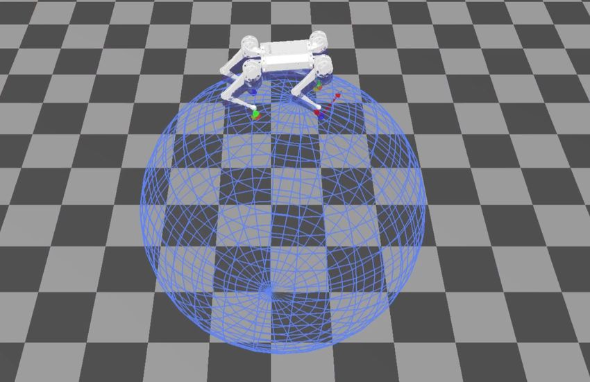
for humans and animals to interact with environments. For Fig. 1: Simulation snapshot of Mini Cheetah dynamically balancing
on and manipulating a ball. The ball has a rigid surface and the
example, manipulation tasks like dribbling a ball, walking on contact force between Mini Cheetah and the ball is represented by
stilts, and playing soccer, all require dexterous legged manip- red arrows. Simulation video is at https://youtu.be/rIVkfudC4 8.
ulation skills with dynamic interaction with the manipulated
object [9], [12], [15]. Not only does this repertoire extend
the scope of robotic manipulation, it also paves the way to In order to address these challenges, we choose a typical
achieve agile locomotion on extremely difficult terrain [17], scenario for analysis in this paper: a quadrupedal robot dy-
for instance, walking on rolling boulders or toppling stepping namically manipulating a ball to follow different trajectories
stones. Enabling legged robots to manipulate objects using while balancing on it, shown in Fig. 1. A Mini Cheetah robot
their legs shows highly dynamic motion ability and pushes [7] and a rigid ball are used and the interaction between them
the limits of robots’ agility and dexterity. is only through contact.
B. Challenges C. Related Work
Dynamic manipulation using legs places several chal- There are several quadrupedal robot platforms developed
lenges with regards to control design: 1) The problem for different tasks including manipulation [5], [6], [10], [13].
involves designing feedback controllers for legged robots to These manipulation tasks are usually achieved by attaching
be able to interact with objects. 2) The manipulated object a manipulator on a legged robot [1], [11]. However, this
is usually unactuated, which increases the degree-of-un- approach does not exploit the ability of legs for manipulation
deractuation of the legged robot. 3) In addition to just tasks.
interacting with the object, the robot is often required to Legs of a quadrupedal robot are used for both manipu-
manipulate the object along a reference trajectory or to lation and locomotion in [14], wherein the legs statically
a desired pose. 4) The manipulation of the object occurs manipulate a box by holding it on both sides. In other
through the locomotion of the robot which is governed by words, two legs function as two manipulators and they do not
the unilateral and friction contact constraints between the simultaneously achieve manipulation and locomotion tasks.
robot and the object. 5) Furthermore, the problem combines A dynamic legged manipulation task has been partially
the challenges of legged locomotion, including hybrid and implemented in [16] for a bipedal robot balancing on and
nonlinear dynamics with high degree-of-underactuation, as manipulating a ball. It consists of a balance controller and
well as challenges of non-prehensile manipulation. a footstep planner but only for 2D implementation. Our
proposed method aims to provide a comprehensive control
The authors are with the Department of Mechanical Engineering, framework for 3D dynamic legged manipulation with appli-
University of California, Berkeley, California, CA 94720, USA cation to Mini Cheetah manipulating a ball.
{yangcyself, bikezhang, zengjunsjtu, ayush.agrawal,
koushils}@berkeley.edu. D. Contribution
This work was partially supported through National Science Foundation
Grant CMMI-1944722. The contribution of this paper is fourfold: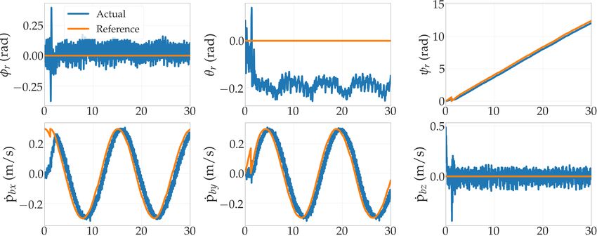
1) Dynamic legged manipulation: We formulate the                 ball is denoted by f , and the generalized torque of the robot
legged manipulation task of a quadrupedal robot dynamically         actuators is represented by τ . Here, we assume that there
manipulating a ball in a systematic way by decoupling the           is no sliding between the ball and the ground, so that we
whole system via contacts.                                          can describe the ball’s motion through its Euler angles as
   2) Interaction model: We develop a simplified interaction        qb ∈ R3 with the ball’s x/y position derived from these
model between a quadrupedal robot and a ball based on the           angles. Note that, with this assumption, we do not have to
concept of equivalent generalized mass.                             consider the force between the ground and the ball, and the
   3) Reaction-force-oriented MPC (R-MPC): We design                gravitation term of the ball can be removed in (2).
a MPC strategy by taking contact forces into account to                For the interaction between the robot and the ball, we also
achieve the goal of dynamic ball manipulation along a given         assume that there is no sliding, so that we have the following
trajectory.                                                         constraints on the acceleration of the contact point,
   4) Foot placement controller: We present a constrained
quadratic program-based foot placement controller which                             J˙r q̇r + Jr q̈r = J˙b q̇b + Jb q̈b .            (3)
adapts to a spherical surface.                                      Substituting Jb† Ab q̈b + Jb† bb + Jb† gb = −f from          (2) and
E. Paper Structure                                                  Jb† J˙r q̇r + Jb† Jr q̈r = Jb† J˙b q̇b + q̈b from (3) into   (1), we
                                                                    have
   This paper is organized as follows. In Sec. II, we introduce
                                                                                                             h
                                                                               Ar q̈r + br + gr + JrT JbT † Ab Jb† (Jr q̈r
the assumptions of the ball and analyze the full dynamics                                                     i                      (4)
with the ball and the simplified dynamics. The proposed                        + J˙r q̇r ) − J˙b q̇b + bb + gb = τ ,
control design is illustrated in Sec. III. In Sec. IV, we present
simulation results for a Mini Cheetah robot. In Sec. V, we          where the Jb† is a pseudo inverse of Jb .
discuss advantages and limitations of our work, and we                 Ignoring the Coriolis force and gravitation terms of the
summarize the paper in Sec. VI.                                     ball bb and gb , and the terms involving the derivatives of
                                                                    Jacobians, we get the equivalent dynamics based on (4) as
                        II. DYNAMICS
                                                                    follows,
   With the goal of dynamically manipulating a ball using                           Ãq̈r + br + gr = τ + JrT f ,           (5)
legs, we analyze the interaction between the robot and the
ball in this section. We first make assumptions of the ball         where à represents the equivalent generalized mass as
model, and then introduce the dynamical model of the robot          follows.
with the ball as well as the simplified model.                                    Ã = Ar + JrT JbT † Ab Jb† Jr .      (6)
   We consider a rigid body model of the ball with the
                                                                    We use this equivalent generalized mass to describe the
following assumptions:
                                                                    dynamics and generate torques in the whole body impulse
  1) The ball does not deform under the influence of external       control (WBIC) which will be introduced in Sec. III-D.
     contact forces.
  2) We know the physical properties of the ball including          B. Simplified Model
     its radius, inertia, and friction parameters.                     Having presented the full dynamics model with consider-
  3) We know the ball’s states including its position and           ation of the ball, we now present a simplified model of the
     velocity.                                                      robot that will be used in the reaction-force-oriented model
  4) There is no slip between the ball and the foot, and the        predictive control (R-MPC) in Sec. III-B. As introduced in
     ball and the ground.                                           [3], we use the lumped mass model,
                                                                                                       nc
A. Dynamics of Cheetah on Ball                                                                         X
                                                                                             mp̈r =          fi + g,                 (7)
   We introduce the robot’s dynamical model with the con-
                                                                                                       i=1
sideration of the interaction with the ball. Rather than solving                                        nc
the dynamical equations of the ball and the robot together,                             d              X
                                                                                           (Iωr ) =          ri × fi ,               (8)
as we will see, we integrate the ball’s effect into the robot’s                         dt             i=1
model. The dynamics of the robot and the ball can be                where pr , ωr , and g are three dimensional vectors denoting
described as follows,                                               the robot’s position, angular velocity, and acceleration due to
                Ar q̈r + br + gr = τ + JrT f ,               (1)    gravity, all in the global frame. The mass and the moment of
                                                                    inertia of the robot are denoted by m and I respectively. nc
                Ab q̈b + bb + gb =    −JbT f ,               (2)
                                                                    is the number of contacts, and ri , fi are the relative position
where qr ∈ R6+nj represents the pose of the floating base           to the center-of-mass and the contact force of the i-th foot,
and the joints of the robot, and nj is the number of joints.        respectively.
qb ∈ R3 represents the pose of the ball, and Ar/b , br/b ,             During the stance phase, as in [3], the MPC makes three
gr/b , Jr/b are the generalized mass matrix, Coriolis force,        assumptions: 1) roll and pitch angles are small, 2) states are
gravitation force and contact Jacobian for robot or ball,           close to the reference trajectory, 3) roll and pitch velocities
respectively. The contact force between the robot and the           are small and off-diagonal terms of the inertia tensors are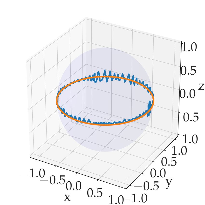
Joint Pos.
Foot Pos. Joint Vel.
Whole Body Impulse Control Joint Torque
Command Foot Placement Controller Joint-level Control
(WBIC) Joint-level
Joint-level control for legs
State Info. Ref. Contact Torque Joint-levelcontrol
controlfor
forlegs
legs
Contact Force Foot Pos. Equivalent
Ref. Contact Force
Generalized [1 kHz]
Ball Reference Contact States
+ Mass
Trajectory
Ref. Vel. Reaction-force-oriented
+ Model Predictive Control Robot Kinematic/ Dynamic Joint Pos.
Contact States Model with Ball Interaction Torque
(R-MPC) Joint Vel.
Contact Force
Body Pos.
[40 Hz] [0.5 kHz]
PD Control for Ball Tracking
Ref. Vel. Ball Pos.
Robot States
Robot Simulator
Fig. 2: Control framework for Mini-Cheetah manipulating a ball along a given ball trajectory. Firstly gait types, reference velocity, contact
forces and the torque to the ball could be given by user or calculated from ball’s reference trajectory. The reaction-force-oriented MPC
computes reference contact forces and foot/body position commands, and this allows us to use WBIC to compute joint torque, position,
and velocity commands, which is sent to each joint controller. The foot placement controller is added to adjust the planned foot placement,
optimizing alternatively with R-MPC. We also consider the interaction between the robot and the ball in the dynamics for WBIC.
small. From [3], the linearized discrete-time dynamics of the and position to drive the ball. The first issue was addressed
system is then expressed as follows, in Sec. II-A, where we analyzed the interaction model and
introduced the equivalent generalized mass. For the second
x(k + 1) = Ak x(k) + Bk f (k) + ĝ, (9) issue, we propose a reaction-force-oriented MPC (R-MPC)
where x represents body configurations and velocities, f (k) and a foot placement controller. The R-MPC is designed to
and ĝ represent the contact forces from the ball and the follow the reference state and contact force, see Sec. III-B.
robot’s gravity. These variables are given by, The foot placement controller first plans the foot placement
according to the Raibert heuristic from [8], and then adjusts
x = [ΘTr pTr ωrT ṗTr ]T , (10) the foot placement point to generate a reference torque to
T the ball, see Sec. III-C. Lastly, the ball reference trajectory
f = [f1 f2 ... fnc ] , (11)
ĝ = [01×3 01×3 01×3 T T
g ] , (12) and PD control for ball tracking, whose commands are used
for R-MPC and the foot placement controller, are described
where Θr is the body orientation. The discrete-time dynam- in Sec. III-E.
ics matrices Ak and Bk are defined as follows, Our control framework is described in Fig. 2. The ball
13×3 03×3 Rz ∆t 03×3
reference trajectory calculates reference velocity, torque and
03×3 13×3 03×3 13×3 ∆t force of the ball according to different scenarios. A PD
Ak = 03×3 03×3 13×3
, (13) controller is added to alter the velocity command, which
03×3
03×3 03×3 03×3 13×3 takes the relative position and velocity of ball and robot into
account. The foot placement controller is at the same level
03×3 ... 03×3 with reaction-force-oriented MPC, sharing the commands
03×3 ... 03×3
and the state information. They work together to track the
Bk = G I −1 [r1 ]× ∆t ... G I −1 [rn ]× ∆t ,
(14)
commands of the reference robot state and the reference
13×3 ∆t/m ... 13×3 ∆t/m contact torque and force to the ball. R-MPC and the foot
where G I is the inertia matrix with respect to the global placement controller optimize the foot placement and the
frame, and Rz is the matrix of the body rotation around z- contact force profile alternatively. The WBIC tracks the foot
axis. [x]× ∈ so(3) is defined as the skew-symmetric matrix position command and the contact force from R-MPC and
for cross products. This discrete-time dynamics is then used the foot placement controller using the interaction model.
in the R-MPC in Sec. III-B. The joint-level control executes commands from WBIC and
controls the motors.
III. C ONTROL D ESIGN
Having presented the assumptions of the ball as well as B. Reaction-force-oriented MPC
the dynamics, we now proceed to present our control design After introducing the control framework, we next present
for dynamic legged manipulation. the reaction-force-oriented MPC (R-MPC), which plans the
contact force with the simplified dynamics from Sec. II-
A. Control Framework B using the reference robot trajectory and the reference
Our proposed control framework extends the control hier- contact force. The R-MPC minimizes the tracking error
archy in [8] by taking two key issues of ball manipulation and the deviation of contact forces, under the friction cone
into account: 1) how to model the quadruped robot balancing constraints. It is a constrained quadratic programming (QP)
on the ball and 2) how to make use of the contact force problem, and its formulation is described as follows,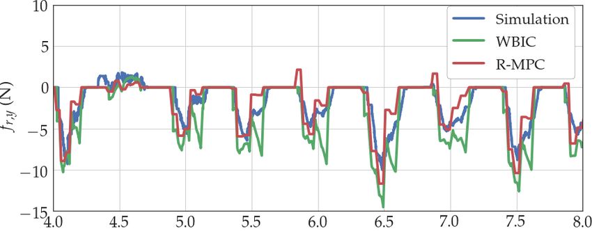
Reaction-force-oriented MPC (R-MPC):
        m
        X
 min          ||x(k + 1) − xref
                            r (k + 1)||Q + ||f (k) − f
                                                       ref
                                                           (k)||R
  x,f
        k=0
s.t.    x(k + 1) = Ak x(k) + Bk f (k) + ĝ,
        |fix (k)| ≤ µf z (x) i = 1 . . . nc ,
        |fiy (k)| ≤ µf z (k) i = 1 . . . nc ,
        fiz (k) ≥ 0           i = 1 . . . nc .                        Fig. 3: Mini-Cheetah on the ball and its zoomed view. The foot
                                                              (15)    placement controller adjusts the swing foot placement after R-MPC
                                                                      by calculating a displacement δpi , so that the torque of the contact
Here Q and R are positive definite weight matrices. The               force at the adjusted foot placement (rbi +δpi )×(−fi −δfi ) meets
friction cone constraint is simplified to a four-side pyramid         the commanded ball torque.
constraining the x/y direction of the force of each i-th contact
fix (k), fiy (k). The R-MPC problem optimizes robot state x
and contact force f that appears as the input to the simplified       and becomes a swing foot, its placement is set according to
system in (9). Different from [3], we consider the reference          the Raibert heuristic from [8] that is presented as follows,
contact forces regulated from the ball’s reference trajectory
in (24), as we hope to control the robot and the ball at the               rcmd
                                                                            i   = pshoulder,i + psymmetry + pcentrifugal ,            (16)
same time. We compute the reference contact force through
a PD control from the ball’s reference trajectory.                    where,
    The reference trajectory xrefr   is similar with [3]. The ref-
                                                                                  pshoulder,i = pr + Rz (ψk ) li ,
erence x/y position of the robot are determined by integrating
                                                                                                tstance
the reference velocities ṗref                                                                          ṗr + k ṗr − ṗref

                             r . The reference yaw and the yaw                    psymmetry =                           r     ,
rate of the robot is from the commanded direction [8]. The                                        s2                                  (17)
z position of the robot is a user defined constant. The other                                     1    h
                                                                                 pcentrifugal   =        ṗr × ωrref .
states (roll, pitch, roll rate, pitch rate, and z velocity) are set                               2    g
to 0.
    The calculation of the reference velocities ṗref r    and the    In (17), li is i-th leg shoulder location with respect to the
reference contact forces f ref (k) will be described in Sec. III-     body frame, and h is the height of the CoM. psymmetry is
E. Besides being passed to WBIC, the solution of f (k) is             called Raibert heuristic that uses foot placements to stabilize
then used as inputs to the foot placement controller, which           the horizontal CoM dynamics, tstance is the stance duration of
will be described next in Sec. III-C. The output of the foot          the current gait cycle, ωrref and ṗref
                                                                                                          r are the reference robot
placement controller affects the relative position of planned         angular and linear velocities respectively.
foot placement ri , which consequently affects the dynamics              After R-MPC plans the contact force profile, the foot
matrix Bk in the next control iteration.                              placement controller alters the foot placement using the
                                                                      following optimization program,
C. Foot Placement Controller
   The foot placement contributes to the torque generated             Foot Placement Controller:
on the ball, so we plan to exploit this potential advantage.
In order to find a foot placement that yields desired torque             min kδτ r (δp , δf )kQr + τbref (δp , δf ) − τb (δp , δf )
                                                                        δp ,δf                                                        Qb
on the ball, the foot placement should ideally be a decision
variable in the R-MPC. However, this makes the optimization                +||δp ||Rδp + ||δf ||Rδf
problem nonconvex, which is computationally expensive to                 s.t. δpi × pbi = 0.
implement in real-time.                                                                                                               (18)
   As a trade-off between the convexity of the optimization
problem and the achievement of the control objective, we              Here, Qr , Qb , Rδp , and Rδf are positive definite weight
formulate the R-MPC and foot placement controller as two              matrices, δp , δf are concatenated vectors of the deviations of
separate optimization problems with the results of one being          contact positions δpi and contact forces δf i of each foot. By
used by the other. Specifically, the R-MPC is solved while            ignoring the higher order terms of infinitesimal variations of
holding the foot placement as a constant. Then, the foot              positions and forces δpi and δf i , we can express the change
placement controller is executed to generate the reference            of the contact torque to robot δτ r , and the contact torque to
foot placement, and the new foot placement will be used in            the ball τb as follows,
the R-MPC in the next control iteration.                                                              4
   The foot placement controller only changes the planned
                                                                                                      X
                                                                                  δτ r (δp , δf ) =         δpi × fi + ri × δf i ,    (19)
foot placement of the swing foot. Once a foot is lifted off                                           i=1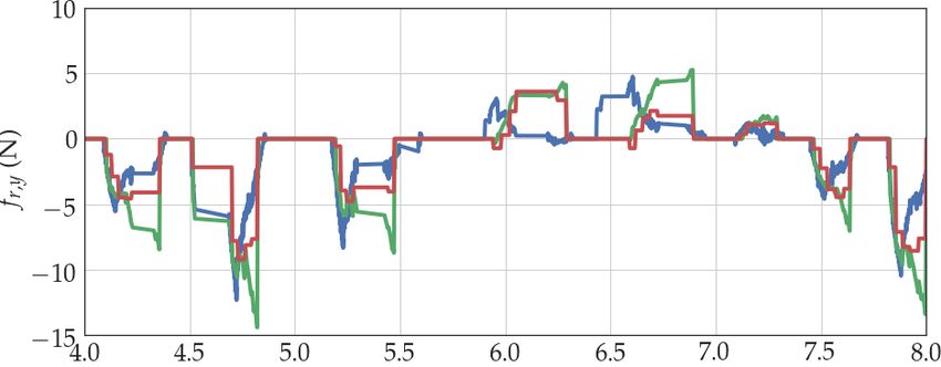
4
X
τb (δp , δf ) = rbi × (−fi ) + δpi × (−fi ) + rbi × (−δf i ).
i=1
(20)
Here, ri and rbi are the relative position from the robot CoM
to foot placement and the relative position from ball’s ground
contact point to the foot placement, respectively. pbi is the
relative position from the ball’s center to the foot contact
point. The contact force fi comes from R-MPC. We illustrate
the geometric relation in Fig. 3. (a) Proposed Controller
The foot placement controller is a multi-objective
quadratic program where the first term minimizes the result-
ing torque change on the robot, and the second term tracks
the reference torque to be applied on the ball. The third
and fourth terms ensure that the solution is in the proximal
neighbor of the original point. The optimization constraint
guarantees that the optimized foot placement is on the surface
of the ball. Note that δf is introduced as a slack variable and
it is not used anywhere else. (b) Baseline Controller
Fig. 4: The comparison of reference speed tracking between (a)
D. Whole-body Impulse Control our proposed controller and (b) the baseline controller. The blue
Following the reference from the foot placement controller line represents the actual speed, which tries to catch up with an
increasing command shown as the orange line.
and the R-MPC, the WBIC tries to incorporate both body
posture stabilization and contact force execution with a full
dynamics model of the robot. Apart from the use of the
The reference x/y velocities of the robot, ṗref
r , are ob-
equivalent generalized mass Ã, we did not make any other
modification to the WBIC described in [8]. The WBIC tained from the reference x/y velocities of the ball ṗref
b and
calculates joint level commands from the reference contact a feedback term, ṗref
PD ,
force and body trajectory in the following steps. First, an ṗref = ṗref + ṗref
r b P D. (22)
acceleration command q̈cmdr of the robot’s configuration is
computed to execute a set of user-specified prioritized tasks. Here, ṗref
PD is a feedback component to minimize the tracking
Then, the following QP is solved, error between the instantaneous ball and the robot positions,
min δf> Q1 δf + δq> Q2 δq ṗref v v
PD = −kp (pr − pb ) − kd ṗr . (23)
δf ,δq
s.t. Sf (Ãq̈r + br + gr ) = Sf Jr> f (floating base dyn.) where pb and pr are the position of the ball and the robot.
ṗr is the velocity of the robot’s CoM.
δq We compute the reference contact force f ref and the
q̈r = q̈cmd
r + (acceleration)
0 nj reference torque τbref through a PD control from ball’s
f = f R-MPC + δf (reaction forces) reference trajectory,
Wf ≥ 0 . (contact force constraints)
f ref (k) = −kpf ep − kdf ev , (24)
(21)
Here, δf and δq are relaxation variables for the reaction
0
forces and the floating base acceleration. Ã, br , gr , Jr are τbref = 0 ×(−kpτ ep − kdτ ev ), (25)
defined in Sec. II-A. The Q, Sf , W are weight matrices of 1
the deviation, the row selection matrix of the floating base,
and the matrix of the friction cone and the normal direction where ep = pref
b − pb and ev = ṗref b − ṗb represent ball’s
of the contact surface. The solution δf is used to adjust position and velocity error. kpf , kdf , kpτ , and kdτ are PD gains.
the planned contact force f to satisfy the full dynamics. At IV. R ESULTS
last, the torque commands can be computed by plugging the
contact forces and the acceleration into the robot’s dynamics Having introduced our control design for dynamic legged
and passed to the joint level controllers. manipulation, we next present simulation results that validate
the control strategy in this section.
E. Ball Reference Trajectory and Tracking
A. Simulation Setup
The ball reference trajectory generates the velocity com-
The simulation environment is set up using the MIT
mand of the robot as well as the reference contact force and
Cheetah Software1 , and a compliant contact model is utilized
the reference torque to be applied on the ball. Note that the
yaw angle of the ball is not considered in the ball reference 1 https://github.com/mit-biomimetics/
trajectory. Cheetah-Software(a) Proposed Controller (a) Proposed Controller
(b) Baseline Controller (b) Baseline Controller
Fig. 5: The comparison of reference ball torque command tracking Fig. 6: The comparison of the contact force tracking in y-direction
between (a) our proposed controller and (b) the baseline controller. between (a) our proposed controller and (b) a baseline controller.
The blue line shows the torque that can be exerted on the ball from Curves shown in the figure are the planned contact force from R-
the R-MPC, which is a cross product of current relative contact MPC (red), the contact force solved in WBIC (green), and the actual
position and the contact force. The orange line is the ball’s torque contact force in simulation (blue)
command from the ball reference trajectory.
the ball reference trajectory, as shown in (25). The blue line
to compute interaction forces between the robot and the shows the torque that can be exerted on the ball from the
ball based on Featherstone’s algorithm [4]. The friction R-MPC and the foot placement controller, which is a cross
coefficient µ is set as 0.9. The ball’s radius is 1m. We product of current relative contact position and the contact
use the controller from [8] that is designed to walk on flat force. While the proposed controller keeps tracking the
ground as our baseline controller. Specifically, the baseline reference commands, the baseline controller loses tracking
controller uses the control framework in Fig. 2 without the and is more noisy.
foot placement controller, with Robot Kinematic/Dynamic Fig. 6 evaluates how MPC and WBIC track the contact
Model of solely the robot, and original MPC instead of R- force command in the same scenario of circular trajectory
MPC. Note that the PD Control for Ball Tracking module is tracking. We only include data from the front left leg,
included and tuned separately in both our proposed controller and other legs are similar. In the control hierarchy, the
and the baseline controller. Also, both the proposed controller contact force from WBIC should follow the command of
and the baseline controller have adapted the direction of R-MPC (proposed controller) or MPC (baseline controller),
gait to the normal direction at the contact point. The ball and by performing the torque commands from WBIC, the
is created from blender [2] with 2562 points. real contact force in simulation is at best to be the same as
B. Performance Evaluation WBIC expected. The closer real contact force to the WBIC’s
command suggests a more accurate dynamic model. Using
The speed tracking performance is shown in Fig. 4. We our proposed controller with equivalent generalized mass, the
set the reference velocity in ball reference trajectory to be a contact force in simulation follows the command of WBIC.
step followed by a ramp, and the yaw rate to be zero. Our However, the contact forces of the baseline controller have
proposed controller can track the reference and continuously larger errors in both timing and scale. Using the proposed
accelerate until 0.75 m/s. The baseline controller can also controller, the mean squared error (MSE) between the real
track a step input but with more tracking errors. Under mild contact force and the WBIC command among four legs
acceleration, the baseline controller maintains stability as of the first 10 seconds is 1810.2, smaller than that of the
well. However, it can not get close to the 0.75m/s speed baseline controller as 2109.4. Note that the commands from
limit, and it has a steady state error for tracking a constant R-MPC/MPC are also different, as the baseline controller
acceleration. The proposed control strategy improves the can not stabilize the robot well.
speed tracking performance and extends the range of speed
for manipulating a ball.
C. Different Scenarios
Fig. 5 shows the effectiveness of our proposed control
design for reference ball torque command tracking. The robot Besides comparing the performance with the baseline con-
manipulates a ball to follow a circular trajectory in this troller, we implement our controller for different scenarios
scenario. The orange line is the ball’s torque command from to further validate our control design.(a) Tracking a straight line (b) Tracking a sinusoid curve (c) Tracking for a circle (d) Yaw angle tracking
Fig. 7: The 3D tracking performance of Mini Cheetah in different scenarios: (a) tracking a straight line (b) tracking a sinusoid curve
(c) tracking a circle (d) orientation tracking. The orange lines are reference trajectories and blue lines are actual trajectories. Red dots
indicate the initial position of the robot. The orientation of the robot is shown as point on an unit sphere in (d).
1) Different Gaits: The proposed controller is tested using V. D ISCUSSION
different gaits. The experimental video shows that trotting,
Ball parameters are important factors affecting the stability
bounding and pronking gaits all work for a Mini Cheetah
and performance of the robot on the ball. The lighter or the
robot dynamically balancing on a ball.
smaller the ball is, the more difficult it is to balance on it.
2) Different Reference Trajectories: Fig. 7 shows the
Our controller can work with more extreme ball parameters.
performance of our proposed control design in four different
Without changing the controller parameters, the minimum
scenarios. In Fig. 7a - 7c, Mini Cheetah manipulates a 2
ball mass and radius for stabilization are 0.5kg and 0.5m,
kg ball to follow a straight line, a sinusoid, and a circle
comparing with the 4kg and 0.8m for the baseline controller.
at velocity 0.3 m/s. Note that the reference yaw angle is
One of the main assumptions that we have made in our
the angle of the robot, rather than the ball. The reference
control design and simulation is the ball’s rigidity. For a
position and velocity in (24) and (25) are generated from
more general case, such as stabilizing Mini Cheetah on a
the ball reference trajectory. For example, for the circular
deformable object, e.g., a fitness ball, we need to take the
trajectory tracking scenario, the ball reference trajectory is
deformation of that object into account during the dynamic
given as,
ref modeling and control design.
pbx r sin(tv ref /r)
pref VI. C ONCLUSION
by −r cos(tv ref /r)
ref = ref , (26)
ṗbx v cos(tv ref /r) In this paper, we have presented a novel control design
ṗref v ref sin(tv ref /r) for dynamic legged locomotion with an application to a
by
quadrupedal robot manipulating a rigid ball. The control
and the robot yaw angle,
design for ball manipulation consists of a reaction-force-
ψrref = tv ref /r, (27) oriented model predictive controller and a foot placement
controller, applied to an interaction model and integrated
where r = 0.7 m is the radius of the circular trajectory, with a nominal WBIC. We numerically verified the control
v ref = 0.3 m/s is the reference velocity, and t is the current strategy with a variety of scenarios. The proposed controller
time. The reference ball velocity ṗref
b in (22) is the reference allows a Mini Cheetah robot to manipulate a ball along
velocity ṗref
bx/y plus a feedback tracking of reference ball straight/sinusoid/circular trajectories and outperforms a base-
position pref
bx/y . Notice that the Mini Cheetah starts with line controller. Experimental results are envisaged for the
position errors from the origin. Fig. 7d shows the orientation future.
of Mini Cheetah following the yaw angle command, which
is illustrated by points on a unit sphere. From these plots, ACKNOWLEDGEMENT
we can clearly see that Mini Cheetah tracks these predefined
The authors would like to thank Professor Sangbae Kim
trajectories well.
and the MIT Biomimetic Robotics Lab for providing the
Fig. 8 shows the detailed tracking errors when Mini
Mini Cheetah simulation software.
Cheetah manipulates a ball to follow a circle: roll, pitch,
yaw angle, ẋ, ẏ, ż of Mini Cheetah. We observe that there
R EFERENCES
is a slight tracking delay on tracking yaw angle and robot
velocities. In order to make the robot move forward, we need [1] E. Ackerman, “Boston dynamics spotmini is all electric, agile, and has
some pitch angle errors to provide torque on the ball and a capable face-arm,” IEEE spectrum, 2016.
[2] B. O. Community, Blender - a 3D modelling and rendering package,
there is a steady state tracking error around 0.2 rad on the Blender Foundation, Stichting Blender Foundation, Amsterdam, 2018.
pitch angle. [Online]. Available: http://www.blender.orgFig. 8: The simulation results of Mini Cheetah manipulating a ball to track a circle. The orange lines are the reference commands, and the
blue lines are the actual values. The first row shows Euler angles (roll φ, pitch θ, and yaw ψ), and the second row shows robot velocities
(ẋ, ẏ, ż).
[3] J. Di Carlo, P. M. Wensing, B. Katz, G. Bledt, and S. Kim, “Dynamic [11] B. U. Rehman, M. Focchi, J. Lee, H. Dallali, D. G. Caldwell, and
locomotion in the mit cheetah 3 through convex model-predictive C. Semini, “Towards a multi-legged mobile manipulator,” in IEEE
control,” in IEEE/RSJ International Conference on Intelligent Robots International Conference on Robotics and Automation, 2016, pp.
and Systems, 2018, pp. 1–9. 3618–3624.
[4] R. Featherstone and K. A. Publishers, Robot Dynamics Algorithm. [12] M. Riedmiller, T. Gabel, R. Hafner, and S. Lange, “Reinforcement
USA: Kluwer Academic Publishers, 1987. learning for robot soccer,” Autonomous Robots, vol. 27, no. 1, pp.
[5] M. Hutter, C. Gehring, D. Jud, A. Lauber, C. D. Bellicoso, V. Tsounis, 55–73, 2009.
J. Hwangbo, K. Bodie, P. Fankhauser, M. Bloesch, et al., “Anymal-a [13] C. Semini, N. G. Tsagarakis, E. Guglielmino, M. Focchi, F. Cannella,
highly mobile and dynamic quadrupedal robot,” in IEEE/RSJ Interna- and D. G. Caldwell, “Design of hyq–a hydraulically and electrically
tional Conference on Intelligent Robots and Systems, 2016, pp. 38–44. actuated quadruped robot,” Proceedings of the Institution of Mechan-
[6] A. M. Johnson and D. E. Koditschek, “Legged self-manipulation,” ical Engineers, Part I: Journal of Systems and Control Engineering,
IEEE Access, vol. 1, pp. 310–334, 2013. vol. 225, no. 6, pp. 831–849, 2011.
[7] B. Katz, J. Di Carlo, and S. Kim, “Mini cheetah: A platform for push- [14] W. Wolfslag, C. McGreavy, G. Xin, C. Tiseo, S. Vijayakumar,
ing the limits of dynamic quadruped control,” in IEEE International and Z. Li, “Optimisation of body-ground contact for augmenting
Conference on Robotics and Automation, 2019, pp. 6295–6301. whole-body loco-manipulation of quadruped robots,” arXiv preprint
[8] D. Kim, J. Di Carlo, B. Katz, G. Bledt, and S. Kim, “Highly dynamic arXiv:2002.10552, 2020.
quadruped locomotion via whole-body impulse control and model [15] J. Z. Wu, S. S. Chiou, and C. S. Pan, “Analysis of musculoskeletal
predictive control,” arXiv preprint arXiv:1909.06586, 2019. loadings in lower limbs during stilts walking in occupational activity,”
[9] X. B. Peng, G. Berseth, K. Yin, and M. Van De Panne, “Deeploco: Annals of biomedical engineering, vol. 37, no. 6, pp. 1177–1189, 2009.
Dynamic locomotion skills using hierarchical deep reinforcement [16] Y. Zheng and K. Yamane, “Ball walker: A case study of humanoid
learning,” ACM Transactions on Graphics, vol. 36, no. 4, pp. 1–13, robot locomotion in non-stationary environments,” in IEEE Interna-
2017. tional Conference on Robotics and Automation, 2011, pp. 2021–2028.
[10] M. Raibert, K. Blankespoor, G. Nelson, and R. Playter, “Bigdog, the [17] M. Zucker, J. A. Bagnell, C. G. Atkeson, and J. Kuffner, “An opti-
rough-terrain quadruped robot,” IFAC Proceedings Volumes, vol. 41, mization approach to rough terrain locomotion,” in IEEE International
no. 2, pp. 10 822–10 825, 2008. Conference on Robotics and Automation, 2010, pp. 3589–3595.You can also read