Each student with their her/his data: understanding sampling distributions
←
→
Page content transcription
If your browser does not render page correctly, please read the page content below
Each student with their her/his data: understanding sampling
                                                                      distributions
                                                                           Mariela Sued(1) , Marina Valdora(1)
arXiv:2105.02727v1 [stat.OT] 6 May 2021

                                                                                         May 7, 2021

                                              (1) Universidad de Buenos Aires and Conicet.

                                          Abstract
                                          Sampling distribution, a foundational concept in statistics, is difficult to understand, since we usually
                                          have only one realization of the estimator of interest. In this work, we present an innovative method for
                                          helping university students understand the variability of an estimator. In our approach, each student
                                          uses a different data set, getting diverse estimations. Then, sharing the results, we can empirically study
                                          the sampling distribution.
                                              After some handmade experiences, we have built a web page to deliver a personalized data set for
                                          each student. Through this web page, we can also reformulate the role of the student in the classroom,
                                          inviting him/her to became an active player, submitting the solution to different problems and checking
                                          whether they are correct. In this work we present a recent experience in such direction.

                                          1     Introduction
                                          A typical problem for users of statistics is to assess the variability of an estimator. As an example, a
                                          couple of years ago, someone came to us with the following problem:
                                              “We reported a median of 3.21 but the referee asked for the error. What should we do? I brought you
                                          this. ”And they gave us the information included in Figure 1: a histogram, the median (3.21), the mean
                                          (4) the standard
                                                         √ deviation of the data (3.40), and en the sample size (n = 120). “For the mean, we know
                                          it. It is 3.40/ 120 ”. As far as we can see, quantifying the variability of an estimator other than the
                                          mean, can usually be counted among these problems. What is going on? Besides knowing the formula
                                          for computing the standard error of the mean, do students really understand what it represents? The
                                          notion of variability associated to data is natural: we have many different values, we can make histograms,
                                          boxplots, etc. But what matters to the referee is the variability of the estimator, the sampling distribution,
                                          for which we only have one realization.
                                             Sampling distribution is one of the most important concept in statistics, fundamental for inference
                                          procedures, like confidence intervals and p-values. Teaching sampling distributions is one of biggest
                                          challenges to be faced in the classroom. Many authors have discussed and written about this issue in recent
                                          years. For instance, Hancock and Rummerfield [2020] have recently described an empirical intervention
                                          which shows that hands-on activity before computer simulation are useful to gain understanding on

                                                                                                1
sampling distribution. In their work the authors present a complete review on the existing literature on
the subject. See also Garfield and Ben-Zvi [2007] and Sotos et al. [2007].
Before going on, we would like to differentiate between two kinds of students: those who have ex-
perience working in a laboratory (students of chemistry, biology and physics) and those who have not
(students of mathematics and computer science, among others). We shall call the former lab students.
After years of teaching, we have realized that lab students are more familiar with the notion of sampling
distribution; they know that each of the students in the lab obtains a different result based on their own
data set. Even though each lab student obtains only one estimation, they know that the student next to
them gets a different estimation and so does each member of the class. If they gathered all the estimates,
they could do descriptive statistics in order to understand the so-called sampling distribution, that is
to say, the distribution of the estimator they are using. Lab students also know that, when reporting
the value of an estimate, it is important to include an “error ”. Typically, they write estimate (error)
, where error is an estimation of the standard deviation of the sampling distribution of the estimator.
For instance, considering the values
√ given above, when they want to inform the mean and its error, they
would express it as 0.31(3.40/ 120).
The last statement is a√consequence of the fact that mathematics gives us a formula for the standard
deviation of the mean: σ/ n, where σ is the standard deviation of the data generating distribution and n
is the sample size. Thanks to this formula, it is easy to report errors when the estimator is the mean: one
simply replaces σ by an estimate such as sd(data), and thus error=sd(data)/sqrt(n). This friendly
formula makes sense even without a deep understanding of its origin. It is related to the variability of
the data and decreases when n increases.
Even though the notion of sampling distribution is clear for lab students, it may not be so for those
who have no experience in the lab, even those who have already worked with real data because they only
observe one data set and therefore they only have one estimate. Our classes do not help much with this
issue; usually our exercises are to be solved based on a data set that is the same for all students. For
example,
A set of 20 lamps from a certain manufacturer has been tested and the following lifetimes have been
obtained (in days).
39.08 45.27 26.27 14.77 65.84 49.64 0.80 66.58 69.60 32.42
228.36 64.79 9.38 3.86 37.18 104.75 3.64 104.19 8.17 8.36
Based on these observations, estimate the mean and the median of the lifetime of a lamp produced
by this manufacturer and the error associated to each estimator.
A good student would do the following:
> mean_estimate mean_estimate
[1] 49.1475
> mean_error mean_error
[1] 11.82242
> median_estimate median_estimate
[1] 38.13
and he would come to ask about the median error. Before answering this question, we want to make
sure they understand the concept of estimation error and, more generally, sampling distribution. In the
following sections we will present our proposal to attain this goal.
22 Our proposal
In order to help the students incorporate the concept of sampling distribution, we invite teachers to
replace the previous type of exercise by a new one in which each student will work based on her own
data. The exercise begins with teachers delivering a data set for each student (or group of students), with
the possibility of changing the sample size. Below, we discuss a form of doing this. Then, the students
compute the estimates of interest based on samples of different sizes. Finally, the teacher collects all the
estimates computed by the class, does descriptive statistics for each sample size and comments on the
results. This kind of activity can be presented at different instances of a statistics course, allowing the
teacher to emphasize concepts of interest at each stage.
In our first implementations of this proposal, we began by printing different data sets in pieces of
paper and handing them out in class. After a successful test trial, we decided to invest time in creating
shiny apps ([Chang et al., 2019]). Shiny apps are a versatile tool that, so far, have allowed us to:
• deliver a different data set to each student, using a personal id number as a seed.
• emulate the process of increasing the sample size by adding more data to the original set.
• give students the possibility to check their answers.
3 An example with shiny
The exercise above should be replaced by
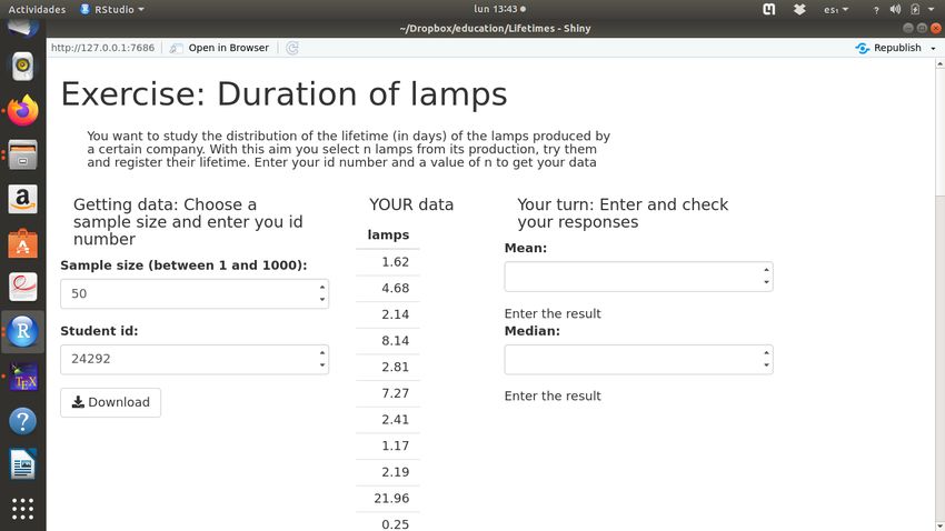
You want to study the distribution of the lifetime (in days) of the lamps produced by a certain company.
With this aim you select n lamps from its production, try them and register their lifetime. To see the
results of your experiment for different values of n click here.
a) For n = 5, n = 30 and n = 100, compute the mean and median lifetime of your data set and check
your results following the instructions on the app.
b) Once you verified the correct answers, for each value of n fill the answers in the following form.
In this way a file will be generated, containing one mean and one median lifetimes for each sample
size (columns) and for each student (rows).
Figure 2 is a screenshot of the webpage the previous link directs you to.
3.1 Working with the mean
In class, we visualize the means reported by the students for each sample size and invite them to identify
their results. Then we draw probability histograms with the means for each sample size with the same
scale in the x axis. Histograms for each required sample size (n = 5, 30, 100) resulting from a class with
80 students are given in Figure 3.
The students are guided to discover that the means are more concentrated as n increases.
Then we discuss the relation between the standard deviation of the means for each sample size and
the error reported by each student.
It should be clear that for large n the error reported by the students are very similar and they are
also similar to the standard deviation of the reported means for the same n.
3This activity should show that the standard error is nothing but an estimation of the standard
deviation of the sampling distribution.
3.2 Working with the median
We repeat the work done for the mean, except that now the students are not able to report an error.
Histograms of the medians for each required sample size (n = 5, 30, 100) resulting from a class with 80
students are given in Figure 4.
At this point we resume the discussion from Section 3.1, where we concluded that the error is nothing
but an estimation of the standard deviation of the sampling distribution. This is the definition of error
and it applies to any estimator; in particular, the median. From Wikipedia:
Definition The standard error of an estimation is the standard deviation (or an estimation) of the
distribution of the estimator.
Based on this definition and the 80 medians obtained by the class, we can compute the standard
error of the median for each sample size by the empirical standard deviation of the set of medians,
namely, if median_5 stores the 80 medians obtained by the students in the class with sample size n = 5,
sd(median_5) can be considered as the required standard error.
In real life, we only have one data set and therefore only one estimation. What we have done here
is unfeasible because we cannot build a histogram with just one datum. However, after doing the type
of exercise we have proposed, students will hopefully understand the notion of sampling distribution and
standard error.
4 Final remarks
The next question is, of course, how to obtain the sampling distribution and the standard error when we
only have one data set. Mathematical statistics proposes different methods to approach this problem,
most of them based on the central limit theorem. On the other hand, an alternative, computer-based
proposal is non-parametric wild bootstrap, which is a way to emulate what we have done in our proposed
exercise but with only one data set. We hope that this kind of classroom work sets the foundations for
understanding resampling methods.
Before concluding, we want to emphasise that the app used to illustrate our proposal is far from
perfect. Since we are not experts in shiny, we understand that this is barely a prototype, than can be
largely improved. For this reason, we decided to share our experience with the community and invite
everyone to create new challenges, making use of the enormous power of Shiny or other applications
that can help to preach our message: individual data sets and active role when interacting with web
applications.
This manuscript was finished while the coronavirus exploded around the word. In-person classes have
been recently cancelled and teachers have been invited to implement virtual teaching. In this context,
we trust that our proposal may help to produce interesting activities.
References
Winston Chang, Joe Cheng, JJ Allaire, Yihui Xie, and Jonathan McPherson. shiny: Web Application
Framework for R, 2019. URL https://CRAN.R-project.org/package=shiny. R package version
1.3.2.
4Joan Garfield and Dani Ben-Zvi. How students learn statistics revisited: A current review of research on
teaching and learning statistics. International statistical review, 75(3):372–396, 2007.
Stacey Hancock and Wendy Rummerfield. Simulation methods for teaching sampling distributions:
Should hands-on activities precede the computer? Journal of Statistics Education, (just-accepted):
1–17, 2020.
Ana Elisa Castro Sotos, Stijn Vanhoof, Wim Van den Noortgate, and Patrick Onghena. Students’
misconceptions of statistical inference: A review of the empirical evidence from research on statistics
education. Educational Research Review, 2(2):98–113, 2007.
5Histogram of data
0.15
0.10
Density
0.05
0.00
0 5 10 15
data
Figure 1: Histogram, median=3.21, mean= 4, sd= 3.40
and n = 120.
6Figure 2:
7n=5 n=30 n=100
1.0
0.25
0.6
0.8
0.20
0.4
0.6
0.15
Density
Density
Density
0.4
0.10
0.2
0.2
0.05
0.00
0.0
0.0
2 4 6 8 10 12 2 4 6 8 10 12 2 4 6 8 10 12
mean mean mean
8
Figure 3: Histograms of means for different values of nn=5 n=30 n=100
1.2
0.5
1.0
0.3
0.4
0.8
0.3
0.2
Density
Density
Density
0.6
0.2
0.4
0.1
0.1
0.2
0.0
0.0
0.0
2 4 6 8 10 12 2 4 6 8 10 12 2 4 6 8 10 12
median median median
9
Figure 4: Histograms of medians for different values of nYou can also read