Effect of spending in the January transfer window

Aadil Shaikh 179048904

 Effect of spending in the January transfer window
 Aadil Shaikh

 Abstract
This paper will investigate how conducting business in the January transfer window changes
the performance of teams in the second half of the season. The league that will be looked at
is the Premier League as this league has the largest influx of money, so ‘smaller’ teams are
also able to spend a high enough amount of money to significantly affect the results of the
findings.

 Introduction
The bi-annual European transfer window came into place in the season of 2002/03 after
many years of debate on whether it would be beneficial for teams. This was set because
without transfer windows, teams were able to buy players at any point in the season, which
led to managers having to coach players who were unsettled. It also shifted the power back
to the coaches and managers, as beforehand players were able to take their foot off the gas
and decide they did not want to play as they thought they would leave the club soon. [1]
The summer and winter transfer windows are both very different in the way they affect
clubs. Choosing to analyse the summer transfer window could have been done, however the
results may be predictable as during summer, there are no competitive league games being
played. This means players bought in have time to adapt to the team, the manager’s tactics
and the environment around them by playing in friendly games during the summer break,
so the likelihood of spending money and having a positive effect on the team’s performance
would be high.
On the contrary, the winter transfer window occurs right in the middle of the season, where
teams are sometimes playing two-three games a week. This means when players are bought
in, they are usually given no time to adapt and are expected to perform at a high level as
soon as they come in. In addition, it is much more difficult to buy players during the winter
transfer window as managers are reluctant to let important players leave halfway through
the season, so clubs are often required to spend a higher amount of money. With all this
uncertainty, it will be interesting to investigate whether carrying out business during the
winter window is beneficial or if it could be better to wait until summer.
The premier league consists of 20 teams, with the champions being the ones who finish first
in the table with the most points, and where the bottom three teams at the end of the
season are relegated to the second division. Clubs are ranked in the table firstly by the
number of points they have accumulated. The points system in the premier league works as
follows:

 • Win = 3 points
 • Draw = 1 point
 • Loss = 0 points

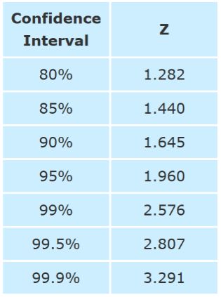
Aadil Shaikh 179048904

So, teams would clearly aim to win as many games as possible to accumulate as many points
as they can. Each team plays every other team in the league twice in a season, once at home
and once away from home. This means there are 38 games played in a season resulting in a
maximum possible points tally of 114. If teams are level on points, their goal difference is
then considered. Goal difference is calculated by
 − 

 Methodology
The money spent by each team in the winter transfer window will be collected and then
compared to the change in league position from game week 20/19 to the final league
position. Game week 20 and 19 are the final game weeks before the January transfer
window begins - depending on which season is looked at - and is approximately halfway
through the season. This was chosen instead of at the end of the transfer window as many
clubs already have deals lined up before the window begins and are simply waiting for the
window to open to complete the deals. This means some deals could be done very early in
the window so these would have to be considered.
The earliest season that will be looked at is the 2014/15 season as this is the final season
from which reliable and accurate data could be collected from. The current season will not
be looked as although the winter transfer window has concluded, there has not been
enough game weeks to analyse any significant change in league position. If a pattern is seen
from the previous seasons, it could allow us to predict the changes in league position for the
current season which will add further evidence to the findings of the paper.
To see whether spending during the transfer window will be significant, a 95% confidence
interval will be carried out comparing amount spent to whether a team moved up in the
table. To calculate the 95% confidence interval, three things must be calculated

 • Number of observations - 
 • Mean - ̅
 • Standard deviation - 
Then, a confidence interval must be chosen which is usually 95%-99%,

As a 95% confidence interval was chosen, the Z value is 1.960. From this, the confidence
 
interval can be calculated by using the formula ̅ ± .
 √

Aadil Shaikh 179048904

This will give the range of values where it is certain to 95% that it contains the mean of the
observed values.

 Initial Outlook

 Table to show change in position relative to money spent in 2018/19 season.

 2018/19 GW 20 Final Change in Money Spent
 Position Position position (m)
 Arsenal 5 5 0 £2.25
 Bournemouth 12 14 -2 £31.32
 Brighton 13 17 -4 £12.51
 Burnley 17 15 2 £30.00
 Cardiff 18 18 0 £18.41
 Chelsea 4 4 0 £64.62
 Crystal Palace 15 12 3 £1.04
 Everton 8 8 0 £0.00
 Fulham 19 19 0 £2.07
 Huddersfield 20 20 0 £1.53
 Leicester 11 9 2 £0.00
 Liverpool 1 2 -1 £0.00
 Manchester City 2 1 1 £6.66
 Manchester United 6 6 0 £0.00
 Newcastle 14 13 1 £22.64
 Southampton 16 16 0 £0.00
 Tottenham 3 4 -1 £0.00
 Watford 9 11 -2 £2.03
 West Ham 12 10 2 £0.00
 Wolverhampton 7 7 0 £18.45
 Wanderers

 Figure 1.1 [1]

 Change in position relative to money spent
 (millions)
 4
 3
 2
 Change in Position

 1
 0
 £0.00 £10.00 £20.00 £30.00 £40.00 £50.00 £60.00 £70.00
 -1
 -2
 -3
 -4
 -5
 Money Spent (millions)

 Figure 1.2

Aadil Shaikh 179048904

Looking at the initial graph for the 2018/19 season it seems there is no clear pattern to
whether the amount of money spent improves the league position by the end of the season.
Only five out of the twenty teams had moved up in the table after January, and one out of
those five teams did not spend anything in the window. Moreover, two teams who spent
more than £10 million moved down in the table. The highest spenders, who spent around
£65 million did not change position after January. This suggests there is no significant
improvement when spending during the January transfer window. However, this is not
mathematically conclusive, so now all the transfers in the past few seasons of the Premier
League will be looked at to see if spending significantly improves league position.

 Inflation
To compare spending from multiple seasons, inflation of the transfer market will need to be
considered. More money seems to be spent every season and the transfer record for a
player also seems to be broken every season. To calculate the rate of inflation, the top 10
most expensive transfers have been collected from every season from each of the top 5
leagues. The top five leagues are the highest tier divisions from England, Germany, France,
Spain and Italy. Although it is only the transfer window in the Premier League being
analysed, inflation in the market is caused by transfers from all the leagues as players are
usually bought from and sold to leagues other than the Premier League.
 Table to show average fee spent in the top 5 leagues [2]
 Seasons Average fee(£m)
 2018/19 41.87
 2017/18 36.39
 2016/17 29.38
 2015/16 23.5
 2014/15 21.41
 Figure 2.1
Once all the data from the past five seasons was collected, the average sum was taken for
each season. However, as this is only an average from the top ten transfers, a linear least
squares approximation was carried out to find a better approximation of the way the
transfer market has changed over the past few seasons.
A linear least squares approximation was used instead of other methods of approximation
such as interpolation as only averages are being used, so the need for the function to be
accurate enough to pass through the data points is not required. Least squares
approximation works by forming a class of functions using the data, and then finding the
function which best minimises the 2 norm of the error. i.e.

 || − ∗ ( )||2 = min || − ( )||2

where ∗ ( ) is the function which minimises 2 norm.
In other words, if there is a data set ( , ), where = 1, … , 

Aadil Shaikh 179048904

 ( ) = ∑ ( )
 =1

Where ( ) are linearly independent basis functions and ( ) are coefficients to be found
which minimise the error. i.e. find such that
 
 2
 ∑( − ( ))
 =1

is minimised.
To calculate this, matrices and vectors were used. The data points were represented as
vectors, where is the vector which contains the points, (year of transfer) and contains
the values (average money spent), so = ( ) = where contains the coefficients to
be found and contains the basis functions ( ). So,
 
 2 2
 ∑( − ( )) = || − ||2
 =1

is what is needed to be minimised. This is minimised if
 . ( − ) = 0
i.e. if the span( ) is orthogonal to the vector − .
The dot product can be represented as
 ( ) ( − ) = ( − ) = 0
But as this is true for any vector , ( − ) = 0 which can be rearranged to give
 = 
And solving this for gave the coefficients for the function to be used. [3]
A different least squares approximation would be given depending on the degree of the
function that is chosen. A quadratic, cubic and quartic function were all attempted and the
one which seemed the best fit was chose.
In the graphs below, the red points are the average fees shown in figure 2.1, and the years
start from 1 (2014/15) to 5 (2018/19).

 Seasons Average fee(£m)
 2018/19 41.87
 2017/18 36.39
 2016/17 29.38
 2015/16 23.5
 2014/15 21.41
 Figure 2.1

Aadil Shaikh 179048904

Quadratic
 ( ) = 0.565 2 + 1.991 + 18.322

 Money spent (m)

 Money spent (m)

 Years
 Figure 2.2
 Money

The function passes through two points and follows the increasing trend of the prices
relatively well, however it does not account for the larger inflation between the third and
fourth season compared to the other seasons.
Cubic

 ( ) = −0.4433 3 + 4.555 2 − 8.4717 + 25.77
 Money spent (m)

 Years
 Figure
 Mone
 2.3
 y
The cubic function also passes through two spent
 points, but better shows the larger inflation
 (m)
between season three and four compared to the other seasons. To see if a higher degree of
the function could be a more accurate estimate,
 Monea quartic function was also made.
 y
 spent
 (m)

 Mone
 y
 spent
 (m)

Aadil Shaikh 179048904

Quartic
 ( ) = −0.9042 4 + 10.4067 3 − 40.2658 2 + 65.1533 − 13.29

 Money spent (m)

 Years
 Figure 2.4
 Mone
Although the quartic function goes throughyall the points, it predicts the market went down
halfway through the fourth season which should
 spent not have happened. The cubic function
seems to follow the pattern the best and so(m)
 seems to be the best fit, so the cubic function is
what was used to calculate inflation of the market.
 Mone
The limitation of the method used was that yas matrices were used, the larger the matrix
was, the closer it would have been to a singular
 spentmatrix, so when carrying out the
 (m)
calculations, accuracy would be lost due to machine precision, which is why a degree of four
was the highest degree that was used. Mone
Using the cubic function y
 spent
 ( ) = −0.4433 3 + 4.555 2 − 8.4717 + 25.77
 (m)
the estimated average transfer fee for each year was taken where (1) was the estimated
average in the season of 2014/15, (2) the estimated average for the season 2015/16 and
so on, giving
 Seasons Average fee (£m)
 2018/19 41.5602
 2017/18 37.6274
 2016/17 27.5212
 2015/16 24.7438
 2014/15 21.1002

 Figure 2.5
To calculate the rate of inflation, the formula used was
 (5)
 100 ( ) − 100
 ( )

where = 1,2, … ,4 where 1 => 2014/15.

Aadil Shaikh 179048904

 Inflation rates calculated from least squares approximation
 Inflation (-2018/19) Inflation rate %
 2014/15 95.56282111
 2015/16 78.17021277
 2016/17 42.51191287
 2017/18 15.05908217
 Figure 2.6
Using the inflation rates, the estimated present value of the transfers were calculated, thus
allowing the data to be analysed.

Linear least squares approximation code
The code used for the linear least squares regression was:
function c = least_sqrs(x, y, d)
% find size of x to see how many seasons are being analysed
n = length(x);
% create a matrix to store basis functions
G = zeros(n, d+1);
% create the basis functions and store them in G
for j = 1:d+1
 for i = 1:n
 G(i,j) = x(i)^(d-(j-1));
 end
end
A = G'*G;
%solve for c to give coefficients
c = A\(G'*y);
end

Where c contains the coefficients of the output function, x is the vector of values, y is the
vector of values and d is the desired degree of the function. This code finds the coefficient
of the function which minimises the 2 norm by via the method proved above by using
matrices and vectors.

 Carrying out a regression analysis
To carry this out, an extra column was created to add a dummy variable, 1 for whether the
team moved up in the table and 0 if the team stayed in the same position or went down.
This was because the initial model would simply measure whether there was a change in
league position, whereas the aim was to see whether the league position of the teams
improved. All the data from the five seasons were analysed together by taking the present
value (as of the 2018/19) season of the previous seasons.

 Figure 3.1
 Regression analysis of the data

Aadil Shaikh 179048904

From the table above, as the 95% confidence interval contains 0 for both variables, neither
of them are significant. More importantly, this means that the amount of money spent does
not significantly improve a team’s position on the table come the end of the season. There
could be several reasons for this; adding on the from reasons mentioned before, some
teams could spend a high amount of money, but only spend it on one player. They may also
bring players in on loan which would mean an initial transfer would not be paid. For these
reasons, now the number of players bought will be looked at to see if it can improve a club’s
position by the end of the season.

 Number of Players bought in
Players can be bought in football in two different ways. They can either be bought or they
can be loaned. Loaning players can essentially be described as `borrowing’ a player from a
team for a certain amount of time – usually around six to twelve months. This allows clubs
to bring in players without paying a transfer fee and are only required to play the player’s
wages. This means players bought in on loan would not have affected the previous model as
a player’s wages was not considered.
Players are usually bought in on loan in winter as a short term `fix’ if the team is desperate
for players. This could be due to injuries to the first team squad or due to summer transfers
not working out as planned. This suggests that by bringing more players in, it should have a
positive short-term effect on the team’s performances, and therefore improving their
league position by the end of the season.
 Table which also shows numbers of players brought in the 2018/19 season
 2018/19 GW 20 Final Change in Money Spent No. of players
 Position Position position (m) brought in
 Arsenal 5 5 0 £2.25 2
 Bournemouth 12 14 -2 £31.32 5
 Brighton 13 17 -4 £12.51 4
 Burnley 17 15 2 £30.00 1
 Cardiff 18 18 0 £18.41 5
 Chelsea 4 4 0 £64.62 3
 Crystal Palace 15 12 3 £1.04 3
 Everton 8 8 0 £0.00 0
 Fulham 19 19 0 £2.07 3
 Huddersfield 20 20 0 £1.53 2
 Leicester 11 9 2 £0.00 3
 Liverpool 1 2 -1 £0.00 0
 Manchester City 2 1 1 £6.66 0
 Manchester United 6 6 0 £0.00 0
 Newcastle 14 13 1 £22.64 3
 Southampton 16 16 0 £0.00 2
 Tottenham 3 4 -1 £0.00 0
 Watford 9 11 -2 £2.03 2
 West Ham 12 10 2 £0.00 1
 Wolverhampton 7 7 0 £18.45 2
 Wanderers
 Figure 4.1

Aadil Shaikh 179048904

Analysis

 Figure 4.2
 Regression analysis of the data
By carrying out another analysis of the number of players bought in compared to whether
the teams position improved, it is clear that the 95% confidence interval contains 0, so the
results show that the number of players bought in does not have a significant impact on
whether a team’s position improves after Christmas . This may be due to many of the
players being bought in may not have had played many games, or they may have been
youth team players who were returning on loan, which may have unfavourably skewed the
data. In addition, some players are merely bought as back up options or to better increase
the competition for places in the squad. This means the players bought in may not have
played most of their games in cup competitions instead of playing in the league games.

 Conclusion
The results have shown that business in the January transfer window does not have any
significant impact on a team as money spent or number of players bought in did not
improve the clubs’ results. One major factor of this is a team’s position in the league at
Christmas is usually a strong representative as to what table will look like come the end of
the season as half the games have already been played. This reduces the likelihood of a
club’s chances of moving up in the table by the end of the season.
Many other factors could have affected the results that were not considered in the model.
Players bought in for high sums of money may have gotten injured for the remainder of the
season meaning they were unable to positively affect the team’s performances. Moreover,
if players are bought from different leagues, it can take time for them to adjust to league so
they may not be able to perform at their best quick enough before the end of the season.
This all suggests that clubs should attempt to carry out all their business during the summer
transfer window, so they are not forced into buying players in winter. They should consider
buying enough players to account for injuries and dips in form of players. However, what
this cannot account for is changes in manager. Usually, if a team performs much worse than
expected, the managers of the club could get sacked resulting in a new manager getting
appointed. When a new manager comes in, clubs can sometimes go through a ‘honeymoon’
period where the new coaching ideas and new freedom can drastically improve a team’s
performance. This can last around 10-15 games, which means consistently changing
managers is also not a very viable option, so again clubs should make sure the team is well
prepared before the season starts during the summer transfer window.

Aadil Shaikh 179048904

 References
 (1) Transfermarkt: latest transfers
 https://www.transfermarkt.co.uk/premier-league/transfers/wettbewerb/GB1
 [Accessed 10th February 2020]
 (2) Premierleague : when did the transfer windows start
 https://www.premierleague.com/news/60258
 [Accessed 7th February 2020]
 (3) Lecture notes: scientific computing - linear least squares approximation
 https://learn-eu-central-1-prod-fleet01-xythos.s3-eu-central-
 1.amazonaws.com/5bfe8efc36910/4040912?response-content-
 disposition=inline%3B%20filename%2A%3DUTF-8%27%27Lecture_Notes_25-11-
 2019.pdf&response-content-type=application%2Fpdf&X-Amz-Algorithm=AWS4-HMAC-
 SHA256&X-Amz-Date=20200224T214837Z&X-Amz-SignedHeaders=host&X-Amz-
 Expires=21600&X-Amz-Credential=AKIAZH6WM4PLYI3L4QWN%2F20200224%2Feu-central-
 1%2Fs3%2Faws4_request&X-Amz-
 Signature=c581db135d0cf6f64cab591eeaa184e139cc91fdb611235687a72bde4e1aac5b
 [Accessed 22nd February 2020]