Nuclear Magnetic Resonance (NMR) Spectroscopy Background Information
←
→
Page content transcription
If your browser does not render page correctly, please read the page content below
1

Nuclear Magnetic Resonance (NMR) Background Information

Instructions for the Operation of the Jeol JNM-GSX 270
FT NMR Spectrometer

               See the Basic Instructions for GC/MS reference on page 49.
         Nuclear Magnetic Resonance (NMR) Spectroscopy
                    Background Information
         There are two main types of nuclear magnetic resonance (NMR) technology that
you will typically encounter in your career as an undergraduate: proton NMR (1H NMR)
and carbon NMR (13C NMR). A 1H NMR works by looking at the change in energy
between the two energy states of protons. These states are affected by the magnetic field,
which is dependent on the electrons around the protons, through the bonds and
corresponding atoms. Chemists can identify a compound by looking at the chemical
shifts produced (Silberberg 624). Chemical shifts result from the “small magnetic fields
that are generated by electrons as they circulate around nuclei” (Skoog 459). This is
essentially the area on a graph where a peak occurs; these peaks are indicative of various
proton interactions within the molecule. By looking at the height of the peak, one is able
to tell the number and types of protons, which subsequently helps identify a particular
compound (Silberberg 624). Examination of charts and tables correlating chemical shifts
to specific functional groups further aids in analyzing NMR spectra (Skoog 463).
Combining all of the aforementioned information enables one to determine a structure for
a compound. The identity of the compound can then be confirmed by comparison to a
known reference.
         A proton is among the easiest nuclei to study due to its atomic number (equal to
one) and also since there are no shielding effects. Due to the spin of this positively
charged proton, a magnetic moment is created. We can use NMR technology to
determine the spin of protons. When the proton is exposed to a magnetic field (as is the
case with NMR), it will orient itself in such a way as to align with or against the magnetic
field (Wade 545). Life, however, is not so simple when looking at complex molecules
and not just protons. Due to electrons in molecules, the nucleus will be shielded; the
electrons will inhibit the nucleus from feeling the full effects of the magnet (Wade 546-
547). Thus shielding should “decrease with increasing electronegativity of adjacent
groups” since the more electronegative groups will withdraw the electrons from adjacent
protons, leaving the nucleus more exposed to the effects of the magnetic field (i.e. less
shielded) (Skoog 461-462). This is where NMR becomes useful. By looking at
shielding, we are able to approximate a structure for a compound (Wade 546-547).
         Carbon NMR is similar to that of proton NMR, but instead looks at the “magnetic
environments of the carbon atoms themselves” (Wade 588). Since the 13C isotope is
relatively rare, 13C NMR is significantly less sensitive than 1H NMR (Wade 589). While
the decreased sensitivity is a disadvantage for carbon NMR, an advantage is that it gives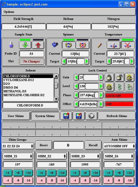
2

us information concerning the backbone of a compound instead of the branches (Skoog
480).
        Something that often gets confusing is the idea of lower and higher fields.
Protons that are less shielded will appear more downfield (lower field). This means that
the peak indicating that proton type will appear farther away from your solvent peak (for
example, CDCl3) and thus have a higher chemical shift number. Protons that are more
shielded will appear closer to the solvent peak (with smaller chemical shift numbers).
This is referred to as being upfield or higher field (Wade 549, 557). Another sometimes
troubling issue is spin-spin splitting. This is when chemical shift peaks split due to the
interaction of one nucleus’s magnetic moment “with the magnetic moments of
immediately adjacent nuclei” (Skoog 460). While NMR technology can be a difficult
concept to grasp, it is a powerful tool in the identification of various compounds and thus
its use will be continued.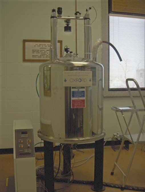
3

             Jeol JNM-GSX 270 FT NMR Spectrometer

Running a Proton NMR

Due to the demand and time it takes to complete NMR’s you should always sign up to
use the instrument in advance.

   •   Upon turning on the monitor, click on the appropriate username to access the
       software necessary to perform NMR experiments.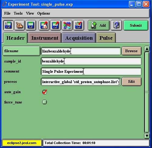
4
• Sign into the NMR logbook.
• Click on the “Delta” icon . A window appears titled “Delta”; this can be
dragged to another location if preferred. This window must be kept open
throughout the entire process or else the program, including all windows, will
close.
Spectrometer Control
o In this window, click on the “Spectrometer Control” button .
Another box labeled “Spectrometer Control” will appear. This box
should now read “No Current Link”.
The bottom of the box should read “eclipse2-FREE-Eclipse 270”.
• Click on this line and hit the “Connect” button.
• When the instrument has connected, the “Queue State”
should show “OWNED”.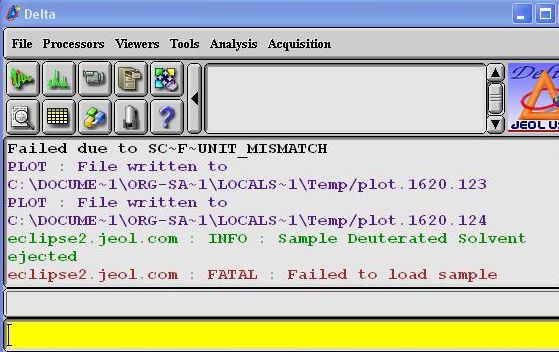
5
In the bottom of this box click on “Sample”.
A box will appear titled “Sample:eclipse2.jeol.com”. A
picture of this window can be seen on page 47.
In the “Sample State” section, make sure that the green
arrow pointing down is highlighted.
¾ Now click on the red arrow pointing up. A clicking
noise should sound from behind you. This indicates
that the sample in the NMR has been ejected.
• Take out the sample from the holder and set it aside.
• Place your sample in the holder at the appropriate level. Wipe off the NMR tube
with a Kimwipe and place the holder with tube in the NMR.
• NEVER PUT THE NMR TUBE IN THE NMR WITHOUT THE HOLDER
AND DON’T PUT THE SAMPLE HOLDER IN THE NMR WITHOUT
THE SAMPLE!!!
• Once you have placed your sample in the NMR, click the arrow pointing down.
• In the “eclipse2.jeol.com” window:
o Make sure the solvent you used is highlighted.
o In the “Lock Control” section, click the “AutoLock & Shim” button .
The fields in this section should turn from red (reading “LockOff” and
“Off”) to yellow (“Autolock & Shim”, “Working”) indicating that the
operations are working.
o DO NOT proceed until “Lock Control” fields are green!
• In the meantime, go to the “Spectrometer Control” window while waiting and
click the “Experiment” button.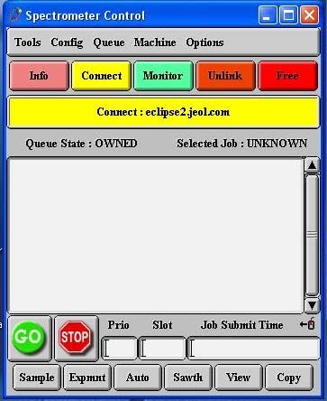
6
o An “Experiment” window will appear. Click on the globe and select
“single_pulse.exp” from the list to the right → OK.
A window with a “Header” tab will appear in the “Experiment
Tool: single_pulse.exp” window. Fill in the filename and sample
ID fields.
Click on the “Autogain” box so that it has a checkmark.
• Once the “Lock Control” fields are green and read “Lock On, Idle”, press
“Submit” on the “Experiment Tool” window.
o An automated voice will ask you to check the sample ID. Do so, and then
press “Acknowledge” or “Go”. If you have not presses “Go” , do so in the
“Spectrometer Control” box.
• The “Delta” window can be used to evaluate the collection progress. The box
will indicate that the job is running and proceed to: the experiment has initialized,
autogain has started, a gain value has been established, and collection has started.
• When the collection has finished, a spectrum will appear.
Running a Carbon NMR
• The instructions for the carbon NMR are the same as for the proton NMR, except
for when setting up the experiment part. While you are waiting for the “Lock
Control” fields to turn green, you click on the globe in the “Experiment” window
and choose the selection: “single_pulse_dec.exp” to set it up for carbon. The
window that will then appear will be “Experiment Tool:single_pulse_dec.exp”.7
Saving/Retrieving Saved Data
• Your file should technically already be saved to the computer from when you
filled in a filename in the “Experiment Tool: single_pulse.exp” window. To
ensure that the file has in fact been saved, go to “File” → “Save As” → click on
the filename you typed before → click OK.
• To save to a disk, go to “File” → “Save As” → change the “Path” to your drive.
The filename should still be in the bottom field since you first saved to the
computer; click OK.
• To retrieve saved data on the computer, go to:
“My Computer” → “Local Disk (C:)” → “Documents & Settings” → the file that
you logged in as user (i.e. Org-Sarkar) → “My Documents” → “Files” →
“Data” → select your file.
o A “Delta” window will appear; this must be kept open during analysis
or all of the subsequent “Delta” windows will be closed.
Analysis
To get rid of the grid lines on the spectrum when viewing and/or printing, press Alt G.
When performing all of the following operations, you can always return to the main view
of the spectrum by clicking Home on the keyboard.
• The important buttons on the top toolbar for analysis are:
o The “Auto Peak Pick” button selects all the peaks on the spectrum,
even ones with almost negligible intensity. It may be more
advantageous in some cases to pick peaks individually rather than use
this tool.
o The “Auto Integrate” button integrates all peaks. As with the peak
picking, doing integration individually may prove more beneficial.
o The “Auto Peak Pick and Integrate” button automatically integrates
and picks all peaks on the spectrum.
• When the “Zoom” button is initiated on the bottom toolbar:
o The “Zoom” button provides a closer view of the spectrum.
Click and drag to create a boxed-in region of the spectrum you
want to zoom in on.
o The “Expand Data” button lengthens or shortens the x-axis.8
o The “Apply Y Gain” button expands or contracts the y-axis making
the peaks appear larger or smaller, respectively.
o has a list of commands that were recently performed. Clicking on a
demand listed will undo it.
• When the “Reference” button is initiated on the bottom toolbar:
o The “Grab Position for Reference” button provides the x coordinates
when you click on this button, click on the spectrum, and then drag.
• When the “Peak” button is initiated on the bottom toolbar:
o The “Peak Pick” button allows you to click on a peak and its location
will be denoted underneath it.
o The “Force Create Peak” button gives a location in ppm of a point
you picked on the spectrum, even if the peak did not exist.
o The “Delete Peak” button deletes the number displayed underneath
the selected peak.
o The “Adjust Peak Threshold” button allows you to click a point on
the graph and a line will be drawn. Peaks above this line will be
automatically picked when using the “Auto Peak Pick” button ;
peaks below the line will not be denoted.
• When the “Integral button” is initiated on the bottom toolbar:
o The “Create Integral” button allows you to manually find the area
under a peak. Click from one part of the peak and drag the cursor to
another point to find the area.
o The “Delete Integral” button is self-explanatory.
o The “Change Slope of Integral” button allows you to move the line
drawn for an integration and results in a different area under the curve.
• When the “Annotation” button is initiated on the bottom toolbar:
o The “Create Text Annotation” button allows you to label peaks or
parts of the graph.9
o The “Edit Text Annotation” button allows you to correct any
mistakes you may have made upon initial typing.
o The “Create Rectangle” button produces a white box that can be
moved to surround peaks or text.
o The “Move/Resize Annotation” button allows you to move text,
boxes, lines, or arrows. If you click on an arrow, line, or box and move
the hand to the corner, squares appear at the edges of the object. Clicking
and dragging the box will resize the object.
o The following functions are self-explanatory but will be mentioned just so
you know what the buttons represent.
Creates a line
Creates an arrow
Creates a double arrow
Deletes an annotation
• When the “PIP” button is initiated on the bottom toolbar:
o The “Create PIP” button allows you to create a picture within a
picture. You can select part of the spectrum and enlarge and move that
portion while keeping the overall spectrum as well.
o These next two button are self-explanatory but are mentioned so you know
what the pictorials represent.
“Move/resize PIP”
“Delete PIP”
• When the “Molecule” button is initiated on the bottom toolbar:
o “Create Molecule” Click on this button and then click and drag it
onto the spectrum; a box will be drawn. A “Select Molecule File” window
will appear. Click on the globe and a list of types of molecules will appear
on the left. Select a type (i.e. amino acid, aromatic, etc.). A different list
of molecules will appear in a box on the right. Select your desired
molecule and press OK. The molecule you selected will be drawn in the
box you created before.
o “Move/resize molecule”10
o “Delete molecule”
• When the “Measure” button is initiated on the bottom toolbar:
o “Create Measure” . Click and drag from one point on the graph to
another. A line is drawn and distances are displayed. This specific button
allows you to create lines that are slanted.
o The “Create Measure in X” button creates a straight horizontal line
between two points.
o The “Create Measure in Y” button creates straight vertical lines
between two points.
o The “Resize Measure” tool allows you to adjust the line length.
o “Resize Measure in X”
o “Resize Measure in Y”
o “Select Measure Near Cursor” . Click the mouse near a line and the
program will automatically denote the line nearest the point where you
clicked.
o “Unselect Measure”
o “Delete Measure”
• When the “Cursor” button is initiated on the bottom toolbar:
o “Create Cursor” allows you to create intersecting lines and will
display the coordinates; more than one cursor can be formed on the graph
at a time.
o “Move Cursor”
o “Select Cursor”
o “Delete Cursor”11
Printing
• To print spectra, click on the “Printer” button on the top toolbar.
• To print a report, click on the “Generate Report” button on the top toolbar.
This will print a peak report of any peak or integral denoted on the spectra.
Closing Down the Instrument
• Go to the “Sample:eclipse2.jeol.com” window and click the up arrow to eject
your sample.
• Remove your sample and replace it with the standard. Place the standard sample
and holder in the NMR, press the green arrow pointing down, and click the
“AutoLock & Shim” button.
• Once the instrument has locked on, click “Unlink” in the “Spectrometer Control”
window. This step is VERY IMPORTANT! It should then indicate that there is
no current link.
• Close all of the windows, including the “Delta” window. Click OK when asked if
you want to exit “Delta”.
• Logout and turn the monitor off.
• Sign out of the logbook.12
“Sample: eclipse2.jeol.com” Window
Eject Sample13
Load Sample
AutoLock & Shim
Lock Control
Fields – Must be
GREEN before
proceeding!
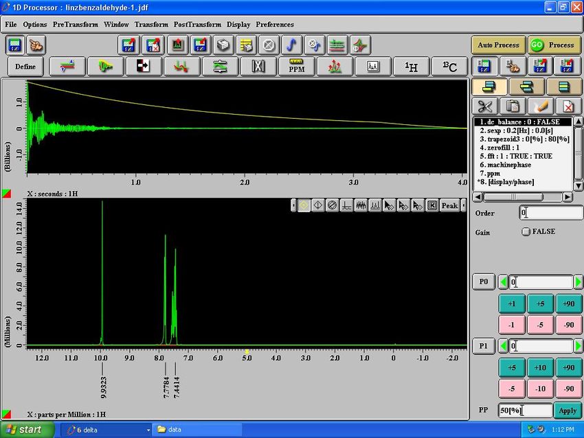
Results for NMR Analysis
Auto peak pick
Auto integrate14
Print spectrum Print report Auto peak pick
& integrate
Downfield
(less shielded) Upfield
(more shielded)
Selected peaks from Bottom analysis toolbar
Type of NMR experiment peak pick mode (zoom, annotate, integrate functions, etc.)
See the NMR Computer Instructions reference on page 49.You can also read