Experimental Comparison of The Two Most Used Vehicle Sideslip Angle Estimation Methods for Model-Based Design Approach

Journal of Physics: Conference Series

PAPER • OPEN ACCESS

Experimental Comparison of The Two Most Used Vehicle Sideslip Angle
Estimation Methods for Model-Based Design Approach
To cite this article: Daniel Chindamo et al 2021 J. Phys.: Conf. Ser. 1888 012006

View the article online for updates and enhancements.

 This content was downloaded from IP address 46.4.80.155 on 08/07/2021 at 05:21

ICMAA 2021 IOP Publishing
Journal of Physics: Conference Series 1888 (2021) 012006 doi:10.1088/1742-6596/1888/1/012006

Experimental Comparison of The Two Most Used Vehicle
Sideslip Angle Estimation Methods for Model-Based Design
Approach

 Daniel CHINDAMO1, *, Marco GADOLA1, Emanuele BONERA1 and Paolo
 MAGRI1
 1
 Department of Industrial and Mechanical Engineering, Automotive Group,
 University of Brescia, I-25123 Brescia, Italy.

 daniel.chindamo@unibs.it

 Abstract. Vehicle sideslip angle estimation is still one of the most challenging research topics
 in the automotive industry. Many papers can be found on this topic, where authors propose
 varied methods to reach the goal. Which is the most effective? After an extensive literature
 review, two very different methods have been identified as the most used: Extended Kalman
 Filter with dynamic model and Artificial Neural Network. In this work a comparison among
 these methods is presented. A fully instrumented car has been used to gather typical vehicle
 dynamics data and feed the models required for a model-based design approach. Results
 showed that each method has either positive aspects or drawbacks.

1. Introduction
Vehicle sideslip angle (VSA) estimation has been a big challenge since the introduction of the very
first on-board active systems controlling vehicle stability, such as the electronic stability control (ESC,
aka ESP) in the early 1990s [1]. It can be used to investigate the cornering behavior in terms of
understeer/oversteer and stability, which are related to active safety and drivability, for either
passenger cars or high-performance vehicles [2]. Moreover, active safety systems such as ESC can be
used in conjunction with VSA estimation in order to extend the vehicle performance envelope and/or
enhance driver perception and comfort [3] as the average driver feels uncomfortable when large VSA
values occur, during emergency maneuvers for instance [4]. It is also worth mentioning that vehicle
drivability is strictly related to VSA: whenever it is large, the authority of the steering wheel angle in
generating a yaw moment becomes significantly reduced. An accurate, reliable and effective VSA
estimation can also be used for autonomous driving strategies and advanced motion control of high-
performance electric vehicles, thus improving active safety and efficiency which are considered key
factors in the automotive market [5].
However, devices required to obtain a direct measure of the vehicle sideslip angle are not robust to
adverse environmental conditions and very expensive as well, therefore they are suitable for R&D
rather than for production vehicles. The VSA hence requires estimation on the basis of conventional
measurements such as lateral/longitudinal acceleration, yaw rate, and steer angle. An estimate of
vehicle speed is also required, to be based in turn on wheel angular speeds.

 Content from this work may be used under the terms of the Creative Commons Attribution 3.0 licence. Any further distribution
 of this work must maintain attribution to the author(s) and the title of the work, journal citation and DOI.
Published under licence by IOP Publishing Ltd 1

ICMAA 2021 IOP Publishing
Journal of Physics: Conference Series 1888 (2021) 012006 doi:10.1088/1742-6596/1888/1/012006

All the above calls for an innovative approach where traditional mechanical engineering skills for
chassis design are integrated with digital knowledge, and the use of innovative tools makes for a
research framework where subjective factors are also taken into account, thus making it also suitable
for the development of Advanced Driver Assistance Systems (ADAS). On top of that, such an
approach recalls what is usually defined as model-based design, where digital models are the key to
product definition. In this case the models related to VSA estimation strategies can be used for
functional simulations at the same time.
VSA estimation is usually classified as Kalman Filter-based and Neural Network-based. According to
[6] however none of the proposed methods succeeded as the most effective, and the problem is not yet
fully resolved. The aim of this paper is to further investigate estimation performances of both methods
through a direct comparison with real-world data.

2. Methods

2.1. Kalman Filter-based estimation
Some It is well known that the Kalman filter (KF) provides optimal state estimation of linear systems.
When dealing with nonlinear systems, as it is often the case in practice, a possible solution to the state
estimation problem is offered by the Extended Kalman Filter (EKF). The EKF is based on a recursive
linearization of the system model around the estimated state so that the KF equations can be applied. A
complete dissertation about the EKF is beyond the scope of this work and the reader may conveniently
refer to [7]. Nevertheless, in order to make the present work more self-contained, the EKF equations
required to estimate the state of a given nonlinear system are reported. Generally speaking, KF (and its
variants) addresses the general problem of trying to estimate the state vector ∈ ℜ of a discrete-
time controlled process that is governed by the generic set of equations [6]. The following system can
be considered:
 = ( − , − , − ) , = ℎ( , ) (1)

where x is the state vector, u the system input, z the system output (the measured variables) and v, w
given Gaussian white noise. Q and R are defined as the system noise w covariance matrix and the
measurement noise v covariance matrix, respectively. Now if the system is linear, (1) can be written in
the form:
 = − + − + − , = + (2)

Denoting with ̂ − the state estimate at step k according to the dynamic evolution of the system (first
equation in (2)), the KF estimation is:
 ̂ − + ( − 
 ̂ = 
 ̂ − ) (3)

One form of K is given in [6]: it depends upon Q and R. For example, if R approaches zero i.e. for an
extremely reliable measurement, then ≈ −1 hence ̂ ≈ −1 . If the system is not linear i.e. it
can be described only in the general form (1), it can be linearized and written in a form similar to (2).
Such an approach is known as an EKF. The vehicle model provides a detailed description of its
dynamic behavior, as it is based on the equilibrium equations. Considering the vehicle as a rigid body,
the following is a generic set of equilibrium equations:
 
 = ( ̇ − ) = ∑ , 
 =1

 = ( ̇ + ) = ∑ =1 , (4)

 ̇ = ∑ =1 

 2

ICMAA 2021 IOP Publishing
Journal of Physics: Conference Series 1888 (2021) 012006 doi:10.1088/1742-6596/1888/1/012006

where m is the vehicle mass, is the polar moment of inertia, , and , are the generic force
contributions along the longitudinal and lateral direction respectively, and is the generic yaw
moment contribution. A dynamic model can feature different levels of detail and complexity and adopt
various assumptions, all these factors affecting the estimation accuracy. For the purpose of this work, a
standard four-wheel model has been used (see Figure 1), while the three equilibrium equations can be
found in [6].

 Figure 1. Dynamic model of a vehicle with road-tyre interaction forces.

2.2. Neural Network-based estimation
The Artificial Neural Network (ANN) approach is the same adopted by Chindamo et al. in [8], using
the Levenberg-Marquardt back-propagation (BP) algorithm along with the mean squared error (MSE)
performance index, as seen in [9]. This BP optimization algorithm updates weights and biases of the
network as presented in [10]. See Figure 2 for the high-level schematics.

 Figure 2. ANN estimation high-level schematics.

The ANN performance is then determined by the MSE which is:
 1 N
 MSE    yi  yk 2
 N i 1
 (5)

where yi and yk are the predicted and target value of the i-th pattern respectively and N is the number of
patterns. The real-world dataset required to train and test the ANN is composed of input data patterns
together with corresponding targets. In this case 90% of the dataset has been used to train the network
while the remaining 10% has been used to test the capability of the network. This is a common
procedure as reported in [11]. The mathematical background along with testing and training
procedures can be found in [10, 11]. For this application inputs (which determine the ANN’s input
layer neuron number) are vehicle speed (Vx), steering angle (), lateral acceleration (ay), longitudinal
acceleration (ax) and yaw rate (r). The output is the VSA (), hence the ANN has only one neuron in

 3

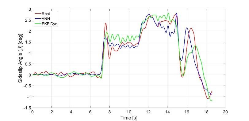
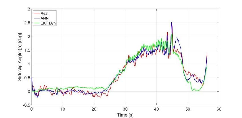
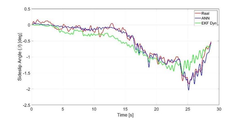
ICMAA 2021 IOP Publishing
Journal of Physics: Conference Series 1888 (2021) 012006 doi:10.1088/1742-6596/1888/1/012006

its output layer. Real-time estimation capabilities of ANNs strictly depend on the number of neurons
in the hidden layer, to be carefully chosen: 10 in this case.
The most challenging part of this work was the identification of an appropriate set of maneuvers to be
used for training. In order to be effective, the training data set should be able to represent the system
and its dynamics in any possible conditions. When this criterion is met, the neuron number of the
hidden layer can be minimized, thus resulting in a simple and light ANN structure [6, 7].
A comprehensive set of demanding maneuvers was designed according to the authors’ experience and
also with an eye on ISO vehicle test standards, and performed as reported in Section 2.3: Step steer
from 30°to 120°steering wheel angle with speed ranging from 60 to 150 kph; 2Hz constant frequency
sine steering (amplitude 60° and 90°) at 60 and 90 kph; 60m and 90m radius steering pad, with
acceleration rate of 5 kph/s. Such data set was employed to train/feed the ANN thus meeting all the
above-mentioned criteria. Therefore, the network can be considered ready for testing with a generic
data set, as shown in Section 3.

2.3. Real-world test and procedures
The car selected for this test was a high-performance road car. All the tests were performed with a
help of a professional test driver at the Nardòproving ground on a flat and dry tarmac surface with a
consistent friction coefficient. Every maneuver was repeated at least three times for statistical purposes.
Both EKF- and ANN-based methods are fed with the basic but critical data set related to vehicle
dynamics, as mentioned in Section 2.2. In order to prove the effectiveness of each method, a
measurement of the VSA (β) is required as well, to be used as a reference and for the purpose of ANN
training. Therefore, a custom set of sensors was designed (see Table 1) and used in conjunction with a
motorsport data logger.

 Table1. List of sensors.
 Sensor Type Range Accuracy
 GPS MoTeC L10 n.a. 0.1 m/s
 Accelerometer Bosch AM600 ±5 G 0,01 G
 Yaw rate sensor YRS3 ±210 deg/s 0,1 deg/s
 Steering (rotary pot.) Gefran PZR20 ±720 deg 0,1 deg
 VSA sensor Correvit S-400 ±60 deg 0,1 deg

3. Results and discussion

This Section reports the comparison between the two VSA estimation methods. Each Figure refers to a
different maneuver and includes the time histories of real-world VSA measured with the optical sensor
(red) and VSA estimation with ANN (blue) and with EKF (green). Figures 3 and 4 represent two of
the so-called steering pad maneuvers in steady state and with different final speed, while Figures from
5 to 8 represent four different step-steer maneuvers with different combinations of speed and target
steering wheel angle.
First of all, as far as the EKF estimation method is concerned, the overall VSA estimation is
considerably accurate. Potential drawbacks are related to the fact that tire/road force interactions
should be modelled through accurate experimental data processed with Pacejka’s well-known magic
formula [6], but unfortunately data available from tire manufacturers might not be accurate enough
quite often. Moreover, the computational effort required by the EKF is fairly high.
Furthermore, it is worth to point out that EKF estimation is quite good in lateral steady state conditions,
while the error in transient conditions is larger. This is related to a state-space vehicle model
composed of four state variables only, in order to limit the computational burden required: yaw rate,
lateral acceleration, lateral forces on front and rear axles [6]. Hence transient maneuvers where
combined lateral and longitudinal forces act on the vehicle at the same time are not fully modelled.

 4

ICMAA 2021 IOP Publishing
Journal of Physics: Conference Series 1888 (2021) 012006 doi:10.1088/1742-6596/1888/1/012006

Finally, the ANN method appears to be the most accurate on both steady-state and transient maneuvers.
This method is also lighter in computational terms since it is based on simple math operations only.
However, as mentioned in Section 2, ANN estimation performances are strictly related to training
quality, which in turn might be highly time and cost demanding. Moreover, the ANN is not able to
consider heavy environmental and system changes such as tires wear and abrupt transition from dry to
wet road surface if they are not explicitly included in the training.

 Figure 3. 90m radius steering pad manoeuvre, speed increasing from 60 to 120 kph.

 Figure 4. 90m radius steering pad manoeuvre, speed increasing from 60 to 100 kph.

 Figure 5. 70°step steer manoeuvre @ 125 kph.

 5

ICMAA 2021 IOP Publishing
Journal of Physics: Conference Series 1888 (2021) 012006 doi:10.1088/1742-6596/1888/1/012006

 Figure 6. 90°step steer manoeuvre @ 125 kph.

 Figure 7. 70°step steer manoeuvre @ 125 kph.

 Figure 8. 90°step steer manoeuvre @ 150 kph.

4. Conclusion

This paper presents a comparison between two different VSA estimation methods, that are the most
popular in vehicle dynamics literature: Kalman Filter and Artificial Neural Network.
All of them have positive aspects and drawbacks: the ANN method can give the best overall
estimation with a low computational burden but it needs a very demanding training procedure,
moreover it is not able to deal with changes of the system and boundary conditions that were not
included in the training. The EKF itself is able to give a good VSA estimation as well but the
computational burden increases with the accuracy of the vehicle model, which requires in turn many
parameters (i.e. tire data) that might be difficult to get. This makes it difficult to use in key
applications such as the typical model-based design approach required by real time operations in state-
of-the-art driving simulators [12].

 6

ICMAA 2021 IOP Publishing
Journal of Physics: Conference Series 1888 (2021) 012006 doi:10.1088/1742-6596/1888/1/012006

References
[1] Van Zanten, A.T., 2000. Bosch ESP systems: 5 years of experience (No. 2000-01-1633). SAE
 Technical Paper.
[2] Marchesin, F.P.; Barbosa, R.S.; Alves, M.A.L.; Gadola, M.; Chindamo, D.; Benini, C. (2016).
 Upright mounted pushrod: the effects on racecar handling dynamics. The Dynamics of
 Vehicles on Roads and Tracks. Proceedings of the 24th Symposium of the International
 Association for Vehicle System Dynamics, IAVSD 2015. 543-552.
[3] Crema, C.; Depari, A.; Flammini, A.; Vezzoli, A.; Benini, C.; Chindamo, D.; Gadola, M.;
 Romano, M. (2015). Smartphone-based system for vital parameters and stress conditions
 monitoring for non-professional racecar drivers. Proceedings of the 2015 IEEE SENSORS.
 7370521
[4] Chindamo D.; Gadola, M.; Marchesin, F.P. Reproduction of real-world road profiles on a four-
 poster rig for indoor vehicle chassis and suspension durability testing. Advances in
 Mechanical Engineering, Vol (9)8, 2017.
[5] Chindamo, D.; Gadola, M. (2018). What is the Most Representative Standard Driving Cycle to
 Estimate Diesel Emissions of a Light Commercial Vehicle? Proceedings of the 1st IFAC
 Workshop on Integrated Assessment Modelling for Environmental Systems, (IAMES 2018),
 May 2018, Brescia, Italy. IFAC-PapersOnLine, 51(5), 73-78.
[6] Chindamo, D.; Lenzo, B.; Gadola, M. (2018). On the vehicle sideslip angle estimation: a
 literature review of methods, models and innovations. Appl. Sci. 2018, 8(3), 355;
 DOI:10.3390/app8030355.
[7] Evensen G. Data assimilation. Berlin Heidelberg: Springer-Verlag; 2009.
[8] Chindamo, D., Gadola, M., Estimation of Vehicle Sideslip Angle Using an Artificial Neural
 Network, 2018, ICMAA 2018 Conference Proceedings, Singapore 24-28 February 2018.
[9] Genta, G. Motor vehicle dynamics: modeling and simulation. World Scientific: Singapore,
 Singapore, 1997.
[10] Levenberg, K., A Method for the Solution of Certain Problems in Least-Squares, Quarterly
 Applied Math. 2, pp. 164-168, 1944.
[11] Marquardt, D., An Algorithm for Least-Squares Estimation of Nonlinear Parameters, SIAM
 Journal Applied Math., Vol. 11, pp. 431-441, 1963.
[12] Emanuele Bonera, Marco Gadola, Daniel Chindamo, Stefano Morbioli, Paolo Magri, Integrated
 Design Tools for Model-Based Development of Innovative Vehicle Chassis and Powertrain
 Systems, International Conference on Design, Simulation, Manufacturing: The Innovation
 Exchange, 09 Sept 2019, Modena, Italy reference.

 7