Extreme Parametric Sensitivity in the Steady-State Photoisomerization of Two-Dimensional Model Rhodopsin - arXiv
←
→
Page content transcription
If your browser does not render page correctly, please read the page content below
Extreme Parametric Sensitivity in the
                                                    Steady-State Photoisomerization of
                                                     Two-Dimensional Model Rhodopsin
arXiv:2011.14342v3 [quant-ph] 9 Jul 2021

                                                                 Chern Chuang∗ and Paul Brumer∗

                                           Chemical Physics Theory Group, Department of Chemistry, and Center for Quantum
                                           Information and Quantum Control, University of Toronto, Toronto, Ontario M5S 3H6,
                                                                                Canada

                                                        E-mail: chern.chuang@utoronto.ca; Paul.Brumer@utoronto.ca

                                                                                   1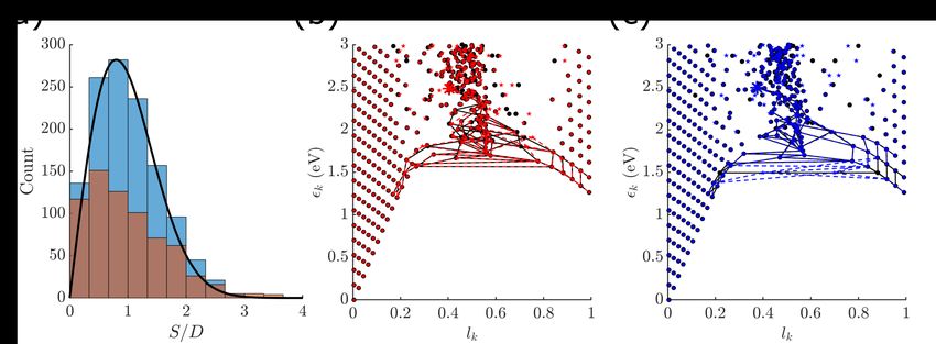
Abstract

     We computationally studied the photoisomerization reaction of the retinal chro-

  mophore in rhodopsin using a two-state two-mode model coupled to thermal baths.

  Reaction quantum yields at the steady state (10 ps and beyond) were found to be con-

  siderably different than their transient values, suggesting a weak correlation between

  transient and steady-state dynamics in these systems. Significantly, the steady-state

  quantum yield was highly sensitive to minute changes in system parameters, while

  transient dynamics was nearly unaffected. Correlation of such sensitivity with standard

  level spacing statistics of the nonadiabatic vibronic system suggests a possible origin

  in quantum chaos. The significance of this observation of quantum yield parametric

  sensitivity in biological models of vision has profound conceptual and fundamental

  implications.

Graphical TOC Entry

                              For Table of Contents Only

                                                2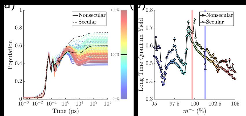
Retinal proteins are a family of important membrane proteins responsible for various
photobiological functions in bacteria and higher life forms. 1–3 Despite the variety of their
functions and the host organisms, the general structure of the retinal proteins is consistent,
i.e. seven transmembrane helices with a retinal chromophore bound to a lysine residue
through a protonated Schiff base. Two systems are frequently studied: (1) rhodopsin that
is found in animal retina, responsible for dim light vision, and (2) bacteriorhodopsin found
in certain bacteria which functions as a light-driven proton pump. In particular, rhodopsin,
with its retinal chromophore initially in an 11-cis conformation, undergoes photoisomeriza-
tion to its all-trans counterpart within 200 fs upon pulsed laser excitation. 4–6 This has been
recently revised to 60 fs. 7 The short reaction time is attributed to a conical intersection
between the ground and excited states, and has been suggested as being responsible for the
high photoisomerization quantum yield (≈67%). 8 These observations have prompted the
important question of the correlation between quantum coherence and biological function.
Our view is clear – such coherences are induced by the laser pulses, and are irrelevant to
nature, which operates with incoherent light. 9,10 Indeed, the natural vision process operates
in the steady state regime.
   Here, we report the observation of a dramatic dependence of the steady-state quantum
yield (QY) on minute changes in system parameters. Our study is based on a two-state
two-mode (2S2M) model coupled to thermal baths initially proposed by Stock et al., 11,12
and later modified/extended to account for numerous experimental observations of bovine
rhodopsin photoisomerization. 7,13 The dependence of the biologically important steady-state
QY on the system parameters is correlated with level spacing statistics, a well established
measure for quantum chaos in molecular systems. This parametric sensitivity has profound
implications for the biology of vision, raising issues as to whether nature’s parameters occupy
a “Goldilocks” region for optimal function.
   This letter is arranged as follows. We first introduce the necessary background and details
of the theoretical treatment, which is followed by a demonstration of the dramatic parametric

                                              3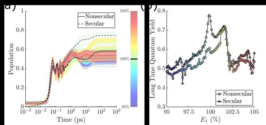
sensitivity of the steady-state photoisomerization QY. We then discuss relationships to quan-
tum chaos, the possibility of experimental measurement of such extreme sensitivity, and its
implications on generic photochemistry in the condensed phase and biological light-sensing.
     Models and Method— The model for the retinal rhodopsin photoisomerization reac-
tion is simulated numerically using the 2S2M model pioneered by Stock et al. 11,12,14 This has
been shown to be an adequate minimal model for studying the photoisomerization dynamics
of retinal chromophores, describing the vibronic structure of a conical intersection. 15 To ac-
count for the environmental effects associated with the protein pocket, the 2S2M system is
further coupled to two sets of harmonic bath modes, and the system dynamics is simulated
using second order quantum master equations.
     A general system-bath Hamiltonian can be written as

                                   H = Hs + Hb + Hsb .                                      (1)

Here, the system (2S2M) Hamiltonian is comprised of two diabatic electronic states |0i and
|1i, a reaction coordinate (coupling mode) φ, and a tuning mode x.

          X                                      ωx2

                                n Vn                                                         0
Hs    =          T̂ + En + (−1)      (1 − cos φ) +     + κxδn,1 δn,n0 + λx(1 − δn,n0 ) |nihn
                                                                                           (2) |
           0
        n,n =0,1
                                  2                 2

where T = −(1/(2m))(∂ 2 /∂φ2 ) + (ω/2)(∂ 2 /∂x2 ) is the kinetic energy operator. All param-
eters, updated in 2017, are obtained from Ref.[ 7 ], and given in Table 1. We define the
range φ ∈ [−π/2, π/2) to be the cis-conformer, and the range φ ∈ [π/2, 3π/2) to be the
trans-conformer. The eigenstates of Hs can be expressed in the direct product space of the
electronic diabatic states {|0i, |1i}, the tuning mode x, and the reaction coordinate φ. 11 The
adiabatic potential energy surfaces are plotted in Fig. 1(a). We note that the protein pocket
of rhodopsin is such that the retinal chromophore is pre-twisted and chiral, which Eq. (2)
does not account for. 16
     A generic property of such a Hamiltonian is that the low energy part of its eigenstates is

                                               4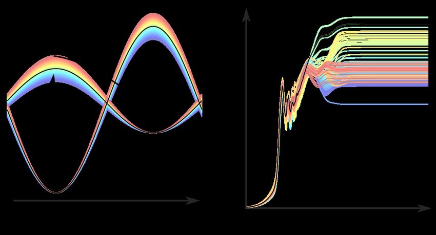
localized in either the cis- or the trans-wells, while higher energy states are more delocalized
over the reaction coordinate φ. 17 To better demonstrate this character, of relevance later
below, we define the following quantity
2π
(1 − cos φ)
Z
1
lk = dφ |hφ|ki|2 · (3)
2π 0 2
where |ki is the k th eigenfunction of the system Hamiltonian Hs , and |φi is the eigenfunction
of the position operator in the reaction coordinate. This quantity is a non-negative real
number with a maximal value of unity. It measures the “trans-ness” of the eigenfunctions:
lk = 0 (1) corresponds to |ki fully localized in the cis- (trans-) well. For intermediate values
it indicates an averaged position of the eigenstate, localized or delocalized. Fig. 1(b) shows
the distribution of lk and eigenstate energies k = hk|Hs |ki. Contribution from the trans
species occurs at most energies, but becomes significant above ∼ 1.4 eV.
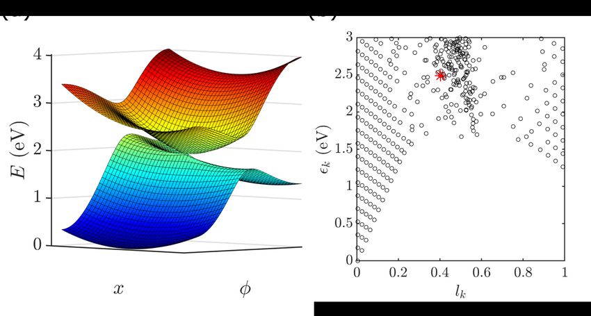
Figure 1: (a) Adiabatic potential energy surfaces of the 2S2M model. (b) The distribution
of the system eigenstates with their energies as the vertical coordinates and lk , defined in
Eq. (3) as the horizontal coordinates. The state that contributes most to the Franck-Condon
state is marked with an asterisk. See text for detailed description.
System-Bath Coupling: To properly account for relaxation effects, the system is coupled
5Table 1: List of parameters, adopted from Ref. [ 7 ]
Parameter Value (eV)
m−1 2.80·10−3
E0 0
E1 2.58
V0 3.56
V1 1.19
w 0.19
κ 0.19
λ 0.19
to environmental degrees of freedom, approximated by the direct product form
X
Hsb = Ŝ (b) ⊗ B̂ (b) , (4)
b
where Ŝ (b) and B̂ (b) are operators that depend only on the system and the bath coordinates,
respectively. The superscript b runs over all system-bath interactions involved. This form of
system-bath interaction Hamiltonian is then treated with the standard Markovian-Redfield
approximation that leads to a quantum master equation, which in the system eigenbasis
reads
∂ X X (b)
ρij = −iωij ρij + Rij,kl ρkl (5)
∂t b kl
X (b) ∗ X (b) ∗
(b) (b) (b)
Rij,kl = −δjl Γirrk + Γljik + Γljik − δik Γlrrj (6)
r r
where ωij is the energy difference between the system eigenstates i and j, and ~ = 1. The
(b)
damping tensors Γijkl are given by
(b) (b) (b)
Γijkl = Sij Skl J (b) (ωkl )n̄BE (ωkl , β), (7)
(b)
where Sij = hi|Ŝ (b) |ji, n̄BE (ω, β) = 1/(eβω − 1) is the Bose-Einstein distribution at inverse
6temperature β = 1/kB T with the Boltzmann constant kB .
The computational cost of propagating the Redfield master equation [Eq. (6)] can be
formidable given that one typically needs up to a thousand lowest energy eigenstates, enough
to converge the Franck-Condon transition from the ground to excited state. Significantly,
this is made more difficult by the fact that we need to examine the long time steady-state
properties, which requires propagating the dynamics up to a nanosecond and beyond. To
this end, one can invoke the Bloch-secular approximation which decouples the population
dynamics from that of the coherences. 14 We compare the results from the full nonsecular
treatment to those of the secular approximation in the next section. (For issues of secular
v.s. nonsecular master equations, see Ref.[ 18 ].)
ωk · b†k bk ,
P
The phonon bath is described within the harmonic approximation, Hph = k
where the system-phonon interaction can be further separated into two components:
Hs−ph = Hs−x + Hs−φ (8)
X
Hs−x = |1ih1| x · gk,x (b†k,x + bk,x ) (9)
k
X
Hs−φ = |1ih1|(1 − cos φ) · gk,φ (b†k,φ + bk,φ ) (10)
k
where gk,x and gk,φ are the coupling strengths of the phonon mode k. It is customary
to represent the summation over the phonon coupling strengths gk as a continuous spectra
density J(ω), taken here in accord with the work of Stock et al., 12,14 to be an Ohmic bath with
exponential cut-off, J(ω) = ηωe−ω/ωc . Couplings to these baths represent the fluctuations
and dissipation of the system dynamics along the modes x and φ.
In the simulation of the retinal photoisomerization, it is customary to choose the initial
condition of the dynamics to be the Franck-Condon state from the ground state located in
the cis-well. 7,11,19 On the other hand, the dynamics initiated from a state similar to the
Franck-Condon state but with all coherence in the energy eigenbasis removed, referred to
as the Franck-Condon mixed state, mimics the effect of an incoherent light source such as
7sunlight. 17 We focus on the dynamics initiated with the Franck-Condon states and compare
the effect of incoherent Franck-Condon mixed initial state in the Supporting Information.
Similar parametric sensitivity was also observed in the non-equilibrium steady state case,
where the retinal system is simultaneously connected to a photon bath describing the in-
coherent sunlight and a phonon bath describing the protein environment. (See Supporting
Information.)
Variation of System Parameters— As noted above, the main result of this work
is our observation of the extreme sensitivity of the steady-state photoisomerization QY to
parameter variation. To demonstrate the extreme sensitivity, consider the results of varying
two representative parameters, as manifest in the computed steady-state QY. First, we
vary the inverse mass m−1 in the kinetic energy term of the reaction coordinate. In the
2S2M model, m−1 determines the characteristic frequency of the reaction coordinate in the
p
harmonic regime, ωφ = k/m and k = V0 /2. It is worth noting that in the original
model of Hahn and Stock 11 m−1 = 4.84 · 10−4 (eV), nearly six-fold smaller than the value
recently suggested by Johnson et al., 7 introduced to reflect the shortening of the rise time of
the trans−photoproduct observed in pump-probe and 2D photon echo measurements with
better temporal resolution. Here we consider ±5% variation of m−1 about the value proposed
by Johnson et al. Note that this corresponds a small change, i.e. ± 2.5%, of the harmonic
frequency along the reaction coordinate.
We have also examined the effect of varying the optical gap between the two diabatic
electronic states, namely the parameter E1 . It is estimated that the inhomogeneous con-
tribution to the broad absorption band of retinal rhodopsin is ∼1000 cm−1 , 20 ∼ 5% of the
optical gap, and which is the range over which we vary the optical gap. To avoid the com-
plication associated with changing the energy storage (E1 − V1 ) and the optical gap of the
trans−product (V0 − E1 + V1 ) when varying E1 we simultaneously change V1 to keep E1 + V1
constant.
Variation of m−1 : Fig. 2(a) shows the time-dependent trans-ground state population of
8the photoisomerization dynamics, which gives the “time-dependent quantum yield”, defined
as the population of diabatic electronic state |1i in the trans−region (π/2 ≤ φ < 3π/2).
The dynamics of the original model with parameters given in Table. 1 is shown in black, and
those with modified m−1 parameters are color-coded. The bath temperature is kept at 0K
to avoid the complication of thermally activated isomerization. Test computations with the
bath at room temperature were also carried out to ensure that the parameter dependences
reported below remained qualitatively unchanged.
Note first that there are signs of coherent beatings at times less than 1 ps reflecting the
fact that the population is oscillating between the reactant and the product wells, as the
population in the cis-well mirrors that of the trans- (data not shown). The photoproduct
appears on the time scale of 100 fs alongside the beatings, in general agreement with ultra-
fast pulsed laser experiments, 4–7 signaling coherent wavepacket dynamics along the direction
of the reaction coordinate φ. While the beatings disappear on the ps time scale, the QY
continues to fluctuate on a far longer time scale, up to 100 ps. This is consistent with
the experimental observations of a closely related system, the photoisomerization of bacteri-
orhodopsin, which shows a similar time-dependent photoproduct signal (up to hundreds of
ps) after the pump pulse. 21 Computationally, the photoproduct signal has a non-monotonic
time dependence, a steep rise on the time scale of 1 ps, followed by a smooth decay until 20
ps, reaching its stationary value at longer times.
Here we are varying the particular system parameter m−1 within the range of ±5% with
respect to the original value. The transient dynamics, up to ∼0.5 ps, show limited m−1
dependence. However, most significantly, the QY at longer times (and hence not observable
in transient dynamics reported in most pulsed laser experiments) depends very sensitively on
m−1 , spanning a wide range between 35% and 75%. This is clearly seen in the QY recorded
at 10 ns as a function of m−1 shown in Fig. 2(b). Note also that Fig. 2 shows both secular
and nonsecular simulations. In general, these two sets of results agree qualitatively with QY
sensitive to the value of m−1 . However, it is clear that the steady-state QY depends on the
9level of treatment for the system-bath interaction.
Figure 2: (a) Time dependent trans-photoproduct population. The full nonsecular dynamics
is shown as solid lines and those of the Bloch-secular are shown with dashed lines. The data
corresponding to the original set of parameters given in Table 1 are shown in black. Data
with varied m−1 are color coded as indicated by the color bar. (b) QY recorded at 10 ns. The
blue and red shaded area correspond to the connectivity graphs shown in Fig. 4, discussed
later below. The bath parameters are adopted from Ref.[ 14 ].
Variation of The Optical Gap: To corroborate the above result and ensure that the
parameter m−1 is not particularly special with regard to the sensitivity of steady-state QY,
we also examined the system dependence on the value of the optical gap. This quantity
is known to be inhomogeneously broadened in natural systems and easier to measure in
concert with the photoisomerization reaction itself. In our case, this amounts to changing
the parameter E1 in the 2S2M model as described in the Models and Method section. The
results are shown in Fig. 3, and are similar to those found in variation of m−1 , i.e. large
variations in QY as a function of small changes in the optical gap.
We also examined other parameters such as ω (the frequency of the harmonic, second
mode in the 2S2M model) and λ (the magnitude of the nonadiabatic coupling, similar to that
studied in Ref.[ 22 ]) and, moreover, two-state-one-mode and two-state-two-mode models with
avoided crossings instead of a conical intersection (parameters given in Ref.[ 14 ]). In light
of recent computational study, 13,23 we simulated and found similar pararmetric sensitivity
10Figure 3: As in Fig. 2, but with E1 is changed instead of m−1 .
in a two-state-three-mode model as well. In addition to the above mentioned nonadiabatic,
two-surface models, we consider a single-surface double well (1S2M) model as well that
is more suitable for describing the adiabatic regime (strong nonadiabatic coupling) of the
isomerization reaction. Details are provided in the Supporting Information. In all cases
similar extreme sensitivities of steady-state QY are found with respect to variations of system
parameters. This suggests that the phenomenon may be an inherent property of the multi-
dimensional vibronic/vibrational systems. 24,25
System Eigenstate Statistics and Relaxation Pathways— We conjecture that
the parametric sensitivity of the steady-state QY results from the sensitivity of chaotic
system dynamics that moves between the two wells and eventually settles into the product
well by relaxation induced by the system-bath coupling. As mentioned in the introduction,
previous studies on similar systems in the quantum chaos literature focus mainly on the
statistical properties of their eigenstates 24 or short-time trajectory-based simulations in the
absence of thermal relaxation. 26,27 The system part in the current study, Eq. (2), falls under
the same category of nonadiabatic vibronic Hamiltonians. 22,24 It is thus expected, if the open
system character is not significant, that similar quantum chaos characteristics would exist
in this system as well. Fig. 1(b) shows the distribution of eigenstates according to their
11energies and lk , a measure of the average position along the reaction coordinate. It is clear
that in the low energy and deeply cis/trans regions (lk → 0 or lk → 1), the distribution of
eigenstates forms a regular grid point lattice. This implies that these states can be written
as direct products of the eigenstates of the two modes, |ki ∝ |nφ i ⊗ |nx i, where nφ and
nx are the quantum numbers of the respective modes. On the other hand, for states with
higher energies and lk closer to 0.5, the grid pattern disappears and the characters of the
two diabatic electronic states and the two modes mix.
The nearest-neighbor spacing distribution (NNSD) of energy eigenstates is a commonly
utilized measure to characterize possible chaotic nature of an isolated system. 22,26 Specifi-
cally, level repulsion tends to imply chaos, most clearly manifest in a Wigner distribution
of adjacent energy level spacings. Here, the procedure described by Haller et al. is used
to account for the smoothly varying part of the density of states. 26 The “unfolded” energy
levels are defined as
i+1 − i
˜i+1 = ˜i + (2k + 1) (11)
j2 +1 − j1
where i are the energies of the eigenstates of Hs with the state index i that runs from 1 to n,
k is a small positive integer defining the locality of the unfolding, j1 = max(1, i − k) and j2 =
min(n−1, i+k). NNSD is the distribution function of S = ˜i+1 −˜i . A non-monotonic NNSD
signals quantum chaotic behavior. Most notably, by assuming linear repulsion between
adjacent levels one arrives at the Wigner distribution for chaotic systems:
πS − πS22
Pw (S) = e 4D (12)
2D2
where D is the mean of the distribution.
The NNSD for our system is shown in Fig. 4(a). It is clear that the distribution is
non-monotonic and near Wignerian and hence chaotic. This is especially true for the higher
energy part of the eigenspectrum (blue), in comparison to the lower energy counterpart
12(brown).
Figure 4: (a) The nearest-neighbor energy level spacing distribution of the model system
studied, using parameters in Table 1. The blue bars (higher) are the 1240 eigenstates taken
from the energy range 4 to 6.4 eV, and the brown ones (lower) are the 686 eigenstates with
energy below 4 eV. The local mean spacing parameter is set to k = 2. The average spacing of
the unfolded levels is D = 1.00 meV. The curve is the Wigner distribution, given in Eq. (12).a
(b) The connectivity tree graph of the systems with m−1 values 99.70% and 99.80% of that
in Table. 1 [red shaded region in Fig. 2(b)], rooted at the brightest state (asterisk). (c) The
tree graph of the systems with m−1 101.3% and 101.4% of that in Table. 1 [blue shaded
region in Fig. 2(b)].
a
The adoption of the higher energy range in Fig. 4(a) is for the purpose of emphasizing the contribution
from the chaotic regime. In all other instances in the paper the photoisomerization dynamics is well converged
by including energy eigenstates below 3 eV.
Quantum chaos in the context of vibronic eigenspectrum of small molecules/ions in the
gas phase has been well established. However, the situation is less clear with systems,
such as ours, coupled to a dissipative environment. As one insightful route, we analyze
the relaxation pathways from the brightest state (the eigenstate contributing the most to
the Franck-Condon state) by examining the Bloch-secular rate matrix elements among the
eigenstates.
In Fig. 4(b) and (c) we show the tree graphs representing the connectivity matrix 28
of the relaxation pathways among system energy eigenstates calculated using two pairs of
m−1 values differed by only 0.1%, corresponding to the red and blue shaded regions shown
in Fig. 2(b), while keeping all other parameters fixed. Each graph shows the eigenstate
distributions [as in Fig. 1(b)] of the two system Hamiltonians with slightly different m−1
13values, using different markers (black filled circles and colored stars). As shown in Fig. 2(b),
the red region corresponds to a parameter regime that shows smooth changes of steady-state
QY with changing m−1 values, whereas the blue region shows dramatic changes. To simplify
the graphs we only connect each higher energy state i to the two lower energy states j with
P (b)
the largest scattering rates b Rjjii in Eq. (6). The connectivity graphs are rooted at the
brightest state of the corresponding systems, defining tree graphs of degree two.
In both pairs of the tree graphs it can be seen that very small changes in m−1 leaves
the approximated direct product structure for states close to the cis- (lk ≈ 0) and the
trans-wells (lk ≈ 1) nearly unaffected. That is, a 0.1% change of m−1 corresponds to a
√
10−3 ≈ 3% change in the harmonic frequency along the reaction coordinate (the vertical
spacing between the lowest and the second lowest symbols), generally not perceivable by
the naked eye. By contrast, a significant portion of the states with lk close to 0.5 shows
a noticeable horizontal shift, signifying the existence of level repulsion discussed above. In
addition, a change in the eigenstate structure induces a dramatic change in the steady-state
QY only if the shifted states are involved in the dominant relaxation pathways. This is so in
the case shown in Fig. 4(c) in contrast to that in Fig. 4(b), in agreement with the respective
behavior of the steady-state QY shown in Fig. 2(b). These observations complement the
parametric sensitivity of long-time dynamics displayed in Figs. 2 and 3, supporting the view
that isolated system chaos propagates through the relaxation dynamics in the open system.
Possible experimental verification— We note the recent work from Schnedermann
et al., where rhodopsins reconstituted with isotope-substituted retinal chromophores show
similar short-time dynamics, but very different steady-state QY. 29 This observation supports
the view that a shorter rise time (the time it takes for the first peak of photoproduct signal
to appear) corresponds to faster reaction, but not necessarily to higher reaction QY. That
is, there is a disconnect between transient and steady state behavior. However, changes with
isotope substitution are not directly comparable to the sensitivity of steady-state QY seen
in Figs. 2 and 3. First, the isotope labelings in these experiments constitute much stronger
14perturbations to the system than those studied here. Second, the experimental observations
are typically, if not exclusively, made on large ensembles of molecules. Within the ensemble,
one expects significant inhomogeneity among the parameters, which would wash out the kind
of parametric sensitivity observed in our computations.
For the real retinal system in an opsin protein pocket, the experimental situation is
expected to be much more complicated than we have modeled above. Indeed, the established
methods of measuring steady-state QY typically involve macroscopic amounts of the sample
being photoisomerized (for example loss of ≈ 10% of the optical density of the reactant over
the course of a few minutes 30,31 ). This being the case, and as noted above, it is likely that the
sensitivity observed here is washed out by the sheer number of retinal molecules in a sample
(≈ 1020 ), each possessing a different conformation. Hence, experimental confirmation of the
sensitivity of QY will require measurements of small ensembles or even of single molecules.
Provided that such sensitivity can be verified experimentally for retinal systems, it may well
be the case that one can find similar phenomena in other light-induced condensed phase
curve-crossing systems.
Open Theoretical Challenges— Additional investigation is needed to clarify the rela-
tionship between quantum chaos and parametric sensitivity of meta-stable state populations
in an open system under environmental dissipation. Whereas we continue to examine a num-
ber of possible measures of quantum chaos for open systems proposed in the literature, such
as the Loschmidt echos and the ratio of eigenvalue differences of the Liouville operator, 32–36
results thus far are inconclusive. (These results are available upon reasonable request.) For
example, they suggest a need for a criteria that applies to open systems whose isolated
system component displays both integrable and chaotic energy level regions. Further, it is
worth noting that our treatment of system-bath interactions is restricted to a Markovian and
perturbative (fast bath) limit, with other environmental effects included as static disorder
(slow bath). In doing so, we do not detect QY sensitivity to the parameters of the system-
bath coupling term or to the bath itself. In the future it would be interesting to examine
15non-pertubative system-bath effects using more sophisticated methods that also account for
the intermediate regime in which the system and the bath time scales overlap. 19,37
Furthermore, while admittedly premature, it is not difficult to suggest a connection be-
tween this result and its possible significant biological implications. That is, does a biologi-
cal light-sensing apparatus benefit from the high sensitivity of the underlying curve-crossing
mechanism to parameter variation? Do the system parameters have to be in a specific
(“Goldilocks”) regime of parameter space? Has natural selection tuned these parameters?
These and related questions warrant further study. What is the key here is the highly sig-
nificant possibility of quantum chaotic contributions and parametric sensitivity in biological
processes and its role in tuning biological function.
Conclusion— The photoisomerization dynamics of retinal chromophore in rhodopsin
was studied using a two-state-two-mode model coupled to dissipative phonon baths. As-
suming the Franck-Condon state as the initial state, the photoproduct (trans-conformer)
populations first show a rapid rise with strong oscillatory features (quantum beats) on the
100 fs time scale. The oscillations then fade out and are replaced by a smooth time-dependent
profile leading to the stationary values on longer time scales. Time-dependent behavior of
this type agrees with available experimental observations of the closely related system bac-
teriorhodopsin, suggesting that simple pictures that correlate short time transient spectral
features with steady-state quantum yield are suspect.
Most significantly, we find that the steady-state quantum yield is highly sensitive to slight
changes in system parameters, while the transient dynamics remains almost unaffected. Such
sensitivity is also observed by changing numerous other parameters of the model system,
suggesting that it is an inherent feature of the nonadiabatic vibronic system studied. Further,
possible experimental measurements of such sensitivity are discussed. The implications of
these results are profound in biological light-sensing systems , and possibly in condensed
phase photochemistry.
Acknowledgement— Support under AFOSR grant FA9550-19-1-0267 is gratefully ac-
16knowledged, as are discussions with Professor Jennifer Ogilvie, University of Michigan and
Professor Arjendu Pattanayak, Carleton College.
Supporting Information
Parametric sensitivity of steady-state photoisomerization observed with incoherent initial
conditions and incoherent excitations, parametric sensitivity and nonsensitivity in single
surface models.
References
(1) Ottolenghi, M. Molecular Aspects of the Photocycles of Rhodopsin and Bacteri-
orhodopsin: A Comparative Overview. Meth. Enzymol. 1982, 88, 470–491.
(2) Wand, A.; Gdor, I.; Zhu, J.; Sheves, M.; Ruhman, S. Shedding New Light on Retinal
Protein Photochemistry. Ann. Rev. Phys. Chem. 2013, 64, 437–458.
(3) Schulten, K. In Quantum Effects in Biology; Mohseni, M., Omar, Y., Engel, G. S.,
Plenio, M. B., Eds.; Cambridge University Press: Cambridge, UK, 2014; Chapter 11,
pp 237–263.
(4) Schoenlein, R.; Peteanu, L.; Mathies, R.; Shank, C. The First Step in Vision: Fem-
tosecond Isomerization of Rhodopsin. Science 1991, 254, 412–415.
(5) Wang, Q.; Schoenlein, R. W.; Peteanu, L. A.; Mathies, R. A.; Shank, C. V. Vibra-
tionally Coherent Photochemistry in the Femtosecond Primary Event of Vision. Science
1994, 266, 422–424.
(6) Polli, D.; Altoè, P.; Weingart, O.; Spillane, K. M.; Manzoni, C.; Brida, D.;
Tomasello, G.; Orlandi, G.; Kukura, P.; Mathies, R. A. et al. Conical Intersection
Dynamics of the Primary Photoisomerization Event in Vision. Nature 2010, 467, 440.
17(7) Johnson, P. J.; Farag, M. H.; Halpin, A.; Morizumi, T.; Prokhorenko, V. I.; Knoester, J.;
Jansen, T. L.; Ernst, O. P.; Miller, R. D. The Primary Photochemistry of Vision Occurs
at the Molecular Speed Limit. J. Phys. Chem. B 2017, 121, 4040–4047.
(8) Dartnall, H. The Photosensitivities of Visual Pigments in the Presence of Hydroxy-
lamine. Vision Res. 1968, 8, 339–358.
(9) Tscherbul, T. V.; Brumer, P. Long-Lived Quasistationary Coherences in a V-type Sys-
tem Driven by Incoherent Light. Phys. Rev. Lett. 2014, 113, 113601.
(10) Brumer, P. Shedding (Incoherent) Light on Quantum Effects in Light-Induced Biolog-
ical Processes. J. Phys. Chem. Lett. 2018, 9, 2946–2955.
(11) Hahn, S.; Stock, G. Quantum-Mechanical Modeling of the Femtosecond Isomerization
in Rhodopsin. J. Phys. Chem. B 2000, 104, 1146–1149.
(12) Hahn, S.; Stock, G. Ultrafast cis-trans Photoswitching: A Model Study. J. Chem. Phys.
2002, 116, 1085–1091.
(13) Marsili, E.; Farag, M. H.; Yang, X.; De Vico, L.; Olivucci, M. Two-State, Three-Mode
Parametrization of the Force Field of a Retinal Chromophore Model. J. Phys. Chem.
A 2019, 123, 1710–1719.
(14) Balzer, B.; Stock, G. Modeling of Decoherence and Dissipation in Nonadiabatic Pho-
toreactions by an Effective-Scaling Nonsecular Redfield Algorithm. Chem. Phys. 2005,
310, 33–41.
(15) González-Luque, R.; Garavelli, M.; Bernardi, F.; Merchán, M.; Robb, M. A.;
Olivucci, M. Computational Evidence in Favor of a Two-State, Two-Mode Model of the
Retinal Chromophore Photoisomerization. Proc. Nat. Acad. Sci. 2000, 97, 9379–9384.
(16) Nakamichi, H.; Okada, T. Crystallographic Analysis of Primary Visual Photochemistry.
Angew. Chem. Int. 2006, 45, 4270–4273.
18(17) Tscherbul, T. V.; Brumer, P. Excitation of Biomolecules with Incoherent Light: Quan-
tum Yield for the Photoisomerization of Model Retinal. J. Phys. Chem. A 2014, 118,
3100–3111.
(18) Dodin, A.; Tscherbul, T.; Alicki, R.; Vutha, A.; Brumer, P. Secular versus Nonsecular
Redfield Dynamics and Fano Coherences in Incoherent Excitation: An Experimental
Proposal. Phys. Rev. A 2018, 97, 013421.
(19) Sala, M.; Egorova, D. Quantum Dynamics of Multi-Dimensional Rhodopsin Photoiso-
merization Models: Approximate versus Accurate Treatment of the Secondary Modes.
Chem. Phys. 2018, 515, 164–176.
(20) Hahn, S.; Stock, G. Femtosecond Secondary Emission Arising from the Nonadiabatic
Photoisomerization in Rhodopsin. Chem. Phys. 2000, 259, 297–312.
(21) Prokhorenko, V. I.; Nagy, A. M.; Waschuk, S. A.; Brown, L. S.; Birge, R. R.;
Miller, R. D. Coherent Control of Retinal Isomerization in Bacteriorhodopsin. Science
2006, 313, 1257–1261.
(22) Fujisaki, H.; Takatsuka, K. Chaos Induced by Quantum Effect due to Breakdown of
the Born-Oppenheimer Adiabaticity. Phys. Rev. E 2001, 63, 066221.
(23) Marsili, E.; Olivucci, M.; Lauvergnat, D.; Agostini, F. Quantum and Quantum-Classical
Studies of the Photoisomerization of a Retinal Chromophore Model. J. Chem. Theo.
Comp. 2020, 16, 6032–6048.
(24) Heller, E. Mode Mixing and Chaos Induced by Potential Surface Crossings. J. Chem.
Phys. 1990, 92, 1718.
(25) Leitner, D. M.; Köppel, H.; Cederbaum, L. S. Statistical Properties of Molecular Spectra
and Molecular Dynamics: Analysis of Their Correspondence in NO2 and C2H4. J.
Chem. Phys. 1996, 104, 434.
19(26) Haller, E.; Köppel, H.; Cederbaum, L. S. On the Statistical Behaviour of Molecular
Vibronic Energy Levels. Chem. Phys. Lett. 1983, 101, 215.
(27) Santoro, F.; Lami, A.; Olivucci, M. Complex Excited Dynamics around a Plateau
on a Retinal-like Potential Surface: Chaos, Multi-Exponential Decays and Quan-
tum/Classical Differences. Theo. Chem. Acct. 2007, 117, 1061–1072.
(28) Biggs, N. Algebraic Graph Theory; Cambridge University Press, 1993.
(29) Schnedermann, C.; Yang, X.; Liebel, M.; Spillane, K.; Lugtenburg, J.; Fernández, I.;
Valentini, A.; Schapiro, I.; Olivucci, M.; Kukura, P. et al. Evidence for a Vibrational
Phase-Dependent Isotope Effect on the Photochemistry of Vision. Nat. Chem. 2018,
10, 449.
(30) Kim, J. E.; Tauber, M. J.; Mathies, R. A. Wavelength Dependent cis-trans Isomeriza-
tion in Vision. Biochem. 2001, 40, 13774–13778.
(31) Sovdat, T.; Bassolino, G.; Liebel, M.; Schnedermann, C.; Fletcher, S. P.; Kukura, P.
Backbone Modification of Retinal Induces Protein-like Excited State Dynamics in So-
lution. J. Amer. Chem. Soc. 2012, 134, 8318–8320.
(32) Grobe, R.; Haake, F.; Sommers, H.-J. Quantum Distinction of Regular and Chaotic
Dissipative Motion. Phys. Rev. Lett. 1988, 61, 1899–1902.
(33) Akemann, G.; Kieburg, M.; Mielke, A.; Prosen, T. Universal Signature from Integra-
bility to Chaos in Dissipative Open Quantum Systems. Phys. Rev. Lett. 2019, 123,
254101.
(34) Sá, L.; Ribeiro, P.; Prosen, T. Complex Spacing Ratios: A Signature of Dissipative
Quantum Chaos. Phys. Rev. X 2020, 10, 021019.
(35) Jalabert, R. A.; Pastawski, H. M. Environment-Independent Decoherence Rate in Clas-
sically Chaotic Systems. Phys. Rev. Lett. 2001, 86, 2490–2493.
20(36) Cucchietti, F. M.; Dalvit, D. A. R.; Paz, J. P.; Zurek, W. H. Decoherence and the
Loschmidt Echo. Phys. Rev. Lett. 2003, 91, 210403.
(37) Chen, L.; Gelin, M. F.; Chernyak, V. Y.; Domcke, W.; Zhao, Y. Dissipative Dynamics
at Conical Intersections: Simulations with the Hierarchy Equations of Motion Method.
Faraday Discuss. 2016, 194, 61–80.
21You can also read