Fiscal and Individual Rates of Return to University Education with and without Graduation
←
→
Page content transcription
If your browser does not render page correctly, please read the page content below
// NO.20-016 | 04/2020

DISCUSSION
     PAPER
  // F R I E D H E L M P F E I F F E R A N D H O LG E R ST I C H N OT H

Fiscal and Individual Rates of
Return to University Education
with and without Graduation
Fiscal and Individual Rates of Return to University Education

                           with and without Graduation

          FRIEDHELM PFEIFFER1,2                         HOLGER STICHNOTH1

                1
                    ZEW– Leibniz Centre for European Economic Research Mannheim
                                  2
                                      University of Mannheim

                                         17 March 2020

                                            Abstract

Based on a detailed model of the German tax-benefit system, this paper simulates private and
fiscal returns to education for college graduates and college dropouts. Completing a five-year
college degree is found to be associated with an internal rate of return (IRR) of 14.2% for gross
earnings, 7.4% for disposable income, and 6.6% for the net fiscal contribution. Individuals who
drop out of college after two years, and subsequently complete a three-year period of vocational
training, are found to have negative IRRs: -0.5% for gross earnings and -5.9% for both dispos-
able income and the net fiscal contribution. In a series of counterfactual experiments, we ex-
plore how these returns react to changes in gross earnings, expenditure per student, and the
level of income tax payments.
Keywords: University education, graduation, dropouts, taxation, internal rate of return
JEL Classification: I26, I28, H23, J31

Acknowledgements: We acknowledge funding by the Federal Ministry of Education and Re-
search, Berlin (project number 01PX16018A). The views expressed in the study are those of
the authors and not necessarily those of the ministry. We would like to thank Sarah McNamara
and Sebastian Siegloch for helpful comments and suggestions.

Address: ZEW – Leibniz Centre for European Economic Research, Mannheim. L 7, 1; 68161

Mannheim, Germany. E-Mail: friedhelm.pfeiffer@zew.de, holger.stichnoth@zew.de.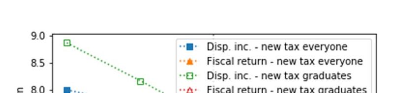
–1–

1     Introduction

While private returns to education have been extensively studied, estimates of the fiscal returns

are relatively scarce. Using a similar methodology to O’Donoghue (1999), Trostel (2010), and

Pfeiffer and Stichnoth (2015), the present paper estimates fiscal returns to education for Ger-

many, based on data from the Socio-Economic Panel (SOEP) for the year 2016 and a detailed

model of the tax-benefit system. The main contribution of this paper is that we estimate fiscal

returns not only for college graduates, but also for college dropouts. The SOEP provides rich

retrospective information which allows us to identify the latter group in the data. We also con-

tribute by using our model for a series of counterfactual experiments, in which we explore how

the returns react to changes in gross earnings, expenditure per student, and the level of income

tax payments.

We find that individuals who drop out of college after two years, and subsequently complete a

three-year period of vocational training, are found to have negative IRRs: -0.5% for gross earn-

ings and -5.9% for both disposable income and the net fiscal contribution. Completing a five-

year college degree is associated with an internal rate of return (IRR) of 14.2% for gross earn-

ings, 7.4% for disposable income, and 6.6% for the net fiscal contribution.

Nonneman and Cortens (1997) estimate fiscal returns to education for Belgium in 1992 and

Trostel (2010) proposes estimates for the United States in the early 2000s. Both studies con-

struct synthetic lifecycles from cross-sectional data and then compute internal rates of fiscal

returns for different educational investments. Using a similar method, the OECD regularly cal-

culates fiscal returns for its member states (e.g., OECD 2019). However, the simulations as-

sume a particular household type (singles without children) and rely on a fairly stylized repre-

sentation of the tax and transfer system. De la Fuente and Jimeno (2009) derive closed-form

expressions for the fiscal returns to education. Their empirical application relies on average

wages and on the assumption that the tax rate remains constant over the lifecycle.
–2–

O’Donoghue (1999) uses a much richer tax-benefit model to simulate fiscal returns for a num-

ber of European countries (Germany, Ireland, Italy, and the United Kingdom) in 1994. Flan-

nery and O’Donoghue (2016) study fiscal returns to education in Ireland over several years.

They do not compute internal rates of returns over the entire (synthetic) lifecycle, but focus on

the marginal fiscal benefit of a hypothetical increase in the years of education for a given

household in a given year. Pfeiffer and Stichnoth (2015) simulate fiscal and individuals returns

to education based on German data for the year 2014. They focus on college graduates and on

individuals who compete a vocational training, but do not study college drop-outs. Their sim-

ulation approach also slightly differs from the one adopted in the present paper.

The rest of the article proceeds as follows. Section 2 defines the measurement of the rate of

return and the simulation scenarios. Section 3 describes the data and the tax-transfer simulation

model. Section 4 presents the results and Section 5 concludes.

2     The Internal Rate of Return and Cost Parameters

Our measure of interest is the internal rate of return (IRR) of an educational investment, which

is defined as the discount rate r at which the present value of the returns equals the present

value of the costs:

                                  1                   1        .                              (1)

    is the return of the investment in period and    its cost, relative to a reference group. Both

revenues and costs are measured on an annual basis. The investment takes             years and the

investment horizon ends in year . For the same educational investment,         and      will differ

depending on whether we study the IRR from the perspective of the individual (in terms of

gross earnings and of disposable income) or from a fiscal perspective. We focus on monetary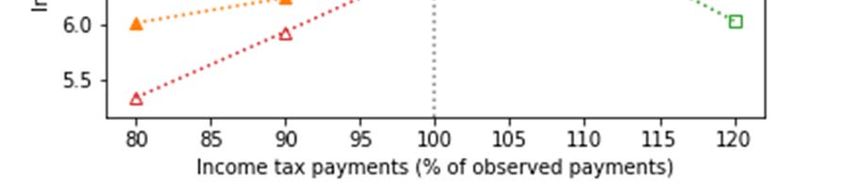
–3–

returns to education, and disregard any spillover effects not operating via the tax-benefit system

(for a discussion of such effects, see Pfeiffer and Stichnoth, 2015).

In this paper we consider individuals with a university-entry qualification and simulate the

average IRR for two investments: completing a five-year university degree1 and attending a

university without graduating. In the latter case, we assume that people drop out after two years

and then complete a three-year period of vocational training. The reference category is made

up of those individuals with a university-entry qualification who never attend a university, but

instead spend three years in vocational training.2 All three educational trajectories (cf. Table 1)

are assumed to begin at age 20.3 The investment horizon ends at age 65, currently the statutory

retirement age.4

Direct costs in the form of school and tuition fees are low in Germany and so we abstract from

these in the calculations. We also abstract from the costs of learning materials. The opportunity

cost of university are the foregone earnings compared to the reference group. For students, we

assume gross earnings of €385 per month (Middendorf et al. 2017); earnings during vocational

training are assumed to be €854 (BIBB 2016). Disposable incomes are computed by subtracting

employees’ social security contributions from these amounts. Income taxation is not relevant

at these low levels of earnings.

1
  In Germany, a successfully completed course of study across all types of university takes an average of 4.7 years
(ABBE 2012), which we round up to five years.
2
  Successful vocational education takes an average of 3.5 years (ABBE 2012). We round this down to 3 years as
we consider only trainees who possess a university entrance qualification. For this group, vocational education,
which includes academic as well as practical training, tends to be shorter.
3
  The average age at which students enroll in university is 19.4 years (ABBE 2018). The average age at the start
of vocational training is 19.5 years (ABBE 2012).
4
  Using a uniform end age is a simplification. While 65 years correspond to the default retirement age for employ-
ees born before 1947, the age is increased to 67 years for employees born after 1964 (with a gradual increase for
the cohorts in between). There are some special rules permitting retirement (with full pension) at age 63 for certain
groups, and the actual retirement age has always been well below the default age of 65. While the simulation
could be refined by experimenting with different retirement ages or by allowing for education-specific retirement
ages, this has little effect on the results because returns that accrue 40 years from now are heavily discounted.

–4–

Table 1: Scenarios

 Age                  No College                     College Dropout               Completed College

 20
                                                        University
 21               Vocational training

 22                                                                                    University

 23            Gross earnings, disposable           Vocational training
            income, and fiscal contributions
 24          simulated based on SOEP data

 26-65         Gross earnings, disposable income, and fiscal contributions simulated based on SOEP data

Public spending per student per year was €7,600 in 2016 (ABBE 2018). In addition, 22% of all

full-time students received benefits under the Federal Training Assistance Act (BAföG). The

average funding amount was €464 per month (ABBE 2018). Half of these benefits are provided

in the form of grants, and the other half in the form of loans. We include only the grant com-

ponent in our measure of fiscal costs. For vocational training, direct fiscal costs are assumed to

be €6,900 per year, the average over all pupils in Germany. These costs arise only for the

school-based component of the training program, as opposed to the training on the job. We

therefore assume that the fiscal cost is incurred only for the first two years of the three-year

period of vocational training.

3        Data and Summary Statistics

Returns and costs that occur once individuals enter the labor market are simulated based on

cross-sectional data from the 2016 wave of the Socio-Economic Panel (cf. Goebel et al. 2018).

We exclude civil servants and the self-employed because for them the structure of both gross

and net earnings is different, owing to special rules regarding social security contributions.
–5–
The breakdown of the number of observations by education and age group is shown in Table
2.5 About 70% of individuals with a college-entry qualification subsequently attended college.
Of these, 84% completed college while 16% dropped out of their studies. The share of dropouts
is about 20% in the youngest and middle age group (25-34 years) and less than 10% for the
oldest group (55-65 years).
Table 2: Summary statistics by age and education
No College College Dropout Completed College
Employ Employ Employ
Gross Gross Gross
Age N ment N ment N ment
earnings earnings earnings
rate rate rate
25-
61 89% €2,819 47 87% €2,525 190 89% €3,385
34
35-
207 91% €2,986 171 88% €3,340 690 93% €4,317
54
55-
88 86% €2,725 55 72% €3,404 557 73% €4,574
65
Total 356 90% €2,894 273 85% €3,209 1,437 86% €4,232
Source: Own calculations based on SOEP 2016. Individuals aged 25 to 65 years (both inclusive) with college‐entry qualifica‐
tions and who are not currently in education. Gross earnings (in EUR per month) conditional on employment.
The employment rate is generally fairly high in the group of people with college-entry qualifi-
cations considered here. In the middle age group (35-54 years), i.e. spanning the twenty years
of prime working age, between 89% and 93% of individuals are employed. The rates are higher
for men and lower for women (not reported here); however, the subsamples are too small to
compute the IRR separately by gender. The employment rates for the youngest age group (the
ten years between ages 25 and 34) are also very high and almost identical for all three education
groups (87-89%). The difference by education is more pronounced for the oldest age group
(the ten years between ages 55 and 65). While 86% of individuals who did not go to college
5
For individuals who do not go to college we simulate labor market biographies starting at age 23 already. In
Table 2, we chose a uniform starting age of 25 for simplicity.–6– are still employed, the share drops to 72% for college dropouts and to 73% for people who completed college. For average gross monthly earnings (conditional on employment), the educational gradient is much steeper. Individuals with no college earn €2,894 per month on average, compared with €3,209 for college dropouts and €4,232 for college graduates. While college graduates earn the most in all age groups, the ranking between people with no college and college dropouts is less clear. Those who never went to college tend to have higher earnings in the youngest age group, but college dropouts earn more, on average, at higher ages. 4 Simulation Methodology While earnings and employment status are directly observed in the data, disposable household income and fiscal contributions have to be simulated. We simulate income taxation, VAT, so- cial security contributions and the key social benefits.6 Taxes and social benefits are simulated at the household level. Since the returns to education are calculated at the individual level, a subsequent back-translation is necessary in couple households. We assume that all tax-transfer variables (including social security contributions for which individual allocation would be pos- sible) are divided equally between both partners. The fiscal returns are computed for the constant policy environment of the year 2018.7 The implicit assumption is that all nominal figures will grow at the rate of inflation and that the system will therefore be stable in real terms. This seems a natural benchmark case; more fun- damental changes in the system (such as the introduction of the Unemployment Benefit II in 2005) have been relatively few and far between and are certainly hard to predict. 6 See Bonin et al. (2016) or Pfeiffer and Stichnoth (2015) for a detailed description of the model. 7 The SOEP data are from 2016 while the tax-benefit rules are for 2018. The difference arises because the data are released with a time lag. Using the 2016 tax-benefit rules instead has little effect on the results.
–7–

The actual work-related expenses, special expenses and extraordinary burdens that can be de-

ducted in the calculation of taxable income are not observed in the SOEP. We therefore assume

that only the statutory deductions apply. We also assume that households claim all benefits

they are entitled to. Finally, when modelling Unemployment Benefit II we take a shortcut by

modelling only the earnings means test and not the wealth test.

We construct synthetic lifecycles for each of our outcome variables based on median values

for each education-age cell. We take five-year moving averages in order to dampen year-to-

year fluctuations and then compute the IRR as defined in Equation (1).8 The entire procedure

is bootstrapped 250 times.

5      Results

Based on gross earnings, the IRR for a college degree is 14.2% (Table 3). The IRR for dispos-

able income is 7.4%, which is considerably lower than for gross earnings. Income taxes, social

security contributions and social transfers thus drive a significant wedge between private gross

and net incentives for investment in education. Nevertheless, both measures point to a substan-

tial private return to a five-year university education.

8
  In some cases, the equation has more than one solution. This happens whenever the series       changes
sign more than once. In these case, we choose the root that is closest to 0 in absolute value.
–8–

Table 3: Returns to education – main specification

                                             No College                College Dropout             Completed College

                                                                             -0.5%                        14.2%
 Gross earnings                           Reference group
                                                                         [-44%; 7.7%]                 [9.8%; 18.3%]
                                                                            -5.9%                         7.4%
 Disposable income                        Reference group
                                                                       [-27.9%; 1.17%]                [4.3%; 9.8%]
                                                                             -5.9%                        6.6%
 Net fiscal contribution                  Reference group
                                                                        [-32.9%; 0.4%]                [3.2%; 9.2%]

Source: Own calculations based on SOEP 2016. Individuals with college‐entry qualifications, excluding civil servants and the
self‐employed. Valid as of tax and transfer rules for 2018. The table reports the median and, in brackets, the 5th and 95th
percentiles over 250 bootstrap runs. Reference group: individuals with college‐entry qualifications who never attend college.

The IRR in terms of the net fiscal contribution is found to be 6.6%.9 This is close to the 6.5%

found by O’Donoghue (1999) for a much earlier year (1994) and to our previous estimates of

5.7% for university versus vocational education (Pfeiffer and Stichnoth, 2015). The OECD

(2019) reports a fiscal IRR for Germany of 9% (men) and 6% (women). With a different meth-

odology, De la Fuente and Jimeno (2009) estimate a fiscal IRR of 4.7% for Germany. The

estimates by Nonneman and Cortens (1997) for Belgium in 1992 are higher (9.6% for men and

12.4% for women). Trostel (2010) finds a fiscal IRR of 10.3% for the US in the early 2000s.

A trajectory in which individuals drop out of college after two years and then complete three

years of vocational training yields a negative IRR for all three outcome measures, compared to

the alternative of directly completing three years of vocational training. In terms of gross earn-

ings, the IRR is -0.5%. For disposable income and the net fiscal contribution, the IRR is -5.9%.

Because of the smaller sample size, the estimates for college drop-outs are less precise than for

college graduates. However, even the 95th percentile of the bootstrap runs is only slightly pos-

itive (0.4%). Despite the large margin of error, the simulation therefore points toward signifi-

cant negative fiscal returns for college drop-outs.

9
  The net fiscal contribution takes VAT and employers’ (in addition to employees’) social security contributions
into account while disposable income does not.
–9–
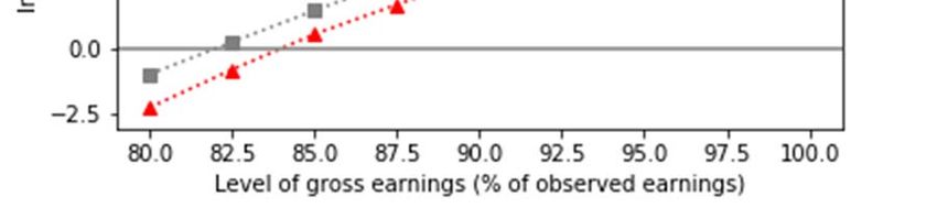
These results are descriptive. To assess the importance of selection effects, we run a counter-
factual experiment in which we vary gross earnings of college graduates by setting them to
between 80% and 100% of their observed level (Figure 1). The selection effect would need to
bring down gross earnings to about 90% of their current level among college graduates in order
to reduce the fiscal IRR to 3%, a value for the discount rate that is often used in the welfare
analysis of government policies (e.g., Hendren and Sprung-Keyser, forthcoming). If gross earn-
ings were only 84% of their current level, the fiscal IRR of a five-year college degree would
become negative. The IRR for gross earnings and disposable income would still be positive in
this case.
Figure 1: Completed college – internal rates of return for counterfactual levels of gross
earnings
Source: Own calculations based on SOEP 2016. Individuals with college‐entry qualifications, excluding civil servants and the
self‐employed. Valid as of tax and transfer rules for 2018. The figure shows how the internal rates of return change if the
gross earnings at each age are scaled down to levels between 80% and 100% of the gross earnings that are actually observed
in the data. The data points represent the median over 250 bootstrap runs.– 10 –
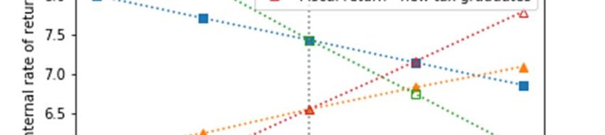
In a second experiment we set the income tax payments to between 80% and 120% of their
actual values (Figure 2). A 20% surcharge for everyone would bring up the fiscal IRR for a
college degree from 6.6% to 7.1%. If the 20% surcharge is paid only by the graduates, the fiscal
IRR reaches 7.8%. The IRR in terms of disposable income is reduced from 7.4% to 6.9% and
6.0%, respectively. Reciprocally, if the income tax payments are scaled down, the IRR in terms
of disposable income goes up while the fiscal IRR is reduced. The effects are roughly linear
over the range considered here.
Figure 2: Completed college – internal rates of return for counterfactual levels of
income tax payments
Source: Own calculations based on SOEP 2016. Individuals with college‐entry qualifications, excluding civil servants and the
self‐employed. Valid as of tax and transfer rules for 2018. The figure shows how the internal rates of return change if the
income tax payments are set to 80%, 90%, 110%, and 120% of their actual value for everyone (filled markers) or for college
graduates only (hollow markers). The data points represent the median over 250 bootstrap runs.
Finally, we use the model for an experiment in which we change the expenditure per student
and simulate the effects on the fiscal IRR for college drop-outs (Figure 3). Even at an expendi-
ture of €5,000 (as opposed to the €8,212 that we assume in our preferred specification), the– 11 –
fiscal return is below -4%. This result is driven by the fact that all individuals complete voca-
tional training after they drop out of college, so their fiscal cost is strictly larger than for the
reference group for any positive expenditure amount.
Figure 3: College dropouts – internal rates of return for counterfactual levels of
expenditure per student
Source: Own calculations based on SOEP 2016. Individuals with college‐entry qualifications, excluding civil servants and the
self‐employed. Valid as of tax and transfer rules for 2018. The figure shows how the internal rates of return change if the
gross earnings at each age are scaled down to levels between 80% and 100% of the gross earnings that are actually observed
in the data. The data points represent the median over 250 bootstrap runs.
6 Conclusion
We provide novel evidence on the returns to education for college drop-outs. From a fiscal
perspective, the return to dropping out is significantly negative, with a point estimate of -5.9%.
By contrast, public investment into college education in Germany yields a fiscal return of 6.6%
if students complete their degree.
Future research should explore the heterogeneity of returns both within and across fields of
study. Courtioux, Grégoir, and Houeto (2014) and Courtioux and Lignon (2016, 2017) develop– 12 –
a dynamic microsimulation model for France to address this issue; they focus on the private
returns to education, however. Finally, while the counterfactual simulations in the present ar-
ticle explore the responsiveness of the fiscal returns to parameters such as gross earnings, the
expenditure per student, and the level of income tax payments, the simulations do not allow for
behavioral adjustments of college enrolment, completion, and labor supply behavior.10 These
margins are important for the optimal design of taxation and human capital policies (cf. Stant-
cheva, 2017, among others).
7 References
ABBE - Autorengruppe Bildungsberichterstattung (2012). Bildung in Deutschland 2012 – Ein
indikatorengestützter Bericht mit einer Analyse zur kulturellen Bildung im Lebenslauf,
Bielefeld.
ABBE - Autorengruppe Bildungsberichterstattung (2018). Bildung in Deutschland 2018 – Ein
indikatorengestützter Bericht mit einer Analyse zu Wirkungen und Erträgen von Bildung,
Bielefeld.
Abramitzky, R. and V. Lavy, V. (2014). How Responsive is Investment in Schooling to
Changes in Redistributive Policies and in Returns? Econometrica, 82(4), 1241-1272.
BIBB – Bundesinstitut für Berufsbildung (2016). Datenreport zum Berufsbildungsbericht 2016
– Informationen und Analysen zur Entwicklung der beruflichen Bildung, Bonn.
Courtioux, P., S. Gregoir, and D. Houeto (2014). Modelling the Distribution of Returns on
Higher Education: A Microsimulation Approach. Economic Modelling, 38, 328-340.
Courtioux, P. and V. Lignon (2016). A Good Career or a Good Marriage: The Returns of
Higher Education in France. Economic Modelling, 57, 221-237.
De la Fuente, A. and J. F. Jimeno (2009). The Private and Fiscal Returns to Schooling in the
European Union. Journal of the European Economic Association, 7(6), 1319-1360.
10
Several quasi-experimental studies have documented reactions along these margins, e.g. Dynarski (2003) and
Abramitzky and Lavy (2014).– 13 –
Dynarski, S. M. (2003). Does Aid Matter? Measuring the Effect of Student Aid on College
Attendance and Completion. American Economic Review, 93, 279-288.
Flannery, D., and O'Donoghue, C. (2016). Utilizing Microsimulation to Estimate the Private
and Fiscal Returns to Education: Ireland 1987–2011. The Manchester School, 84(1), 55-
80.
Goebel, J., M. M. Grabka, S. Liebig, M. Kroh, D. Richter, C. Schröder and J. Schupp (2019).
The German Socio-Economic Panel (SOEP). Jahrbücher für Nationalökonomie und
Statistik, 239(2), 345-360.
Hendren, N. and B. Sprung-Keyser (forthcoming): A Unified Welfare Analysis of Government
Policies. Quarterly Journal of Economics.
Middendorff, E., B. Apolinarski, K. Becker, P. Bornkessel, T. Brandt, S. Heißenberg and J.
Poskowsky (2017). Die wirtschaftliche und soziale Lage der Studierenden in Deutschland
2016. 21. Sozialerhebung des Deutschen Studentenwerks – durchgeführt vom Deutschen
Zentrum für Hochschul- und Wissenschaftsforschung. Berlin: Bundesministerium für Bil-
dung und Forschung (BMBF).
Nonneman, W. and I. Cortens (1997). A Note on the Rate of Return to Investment in Education
in Belgium. Applied Economics Letters, 4(3), 167-171.
O'Donoghue, C. (1999). Estimating the Rate of Return to Education using Microsimulation.
Economic and Social Review, 30(3), 249-266.
Pfeiffer, F. and H. Stichnoth (2015), Fiskalische und individuelle Bildungsrenditen – aktuelle
Befunde für Deutschland, Perspektiven der Wirtschaftspolitik 16(4), 393-411.
OECD (2019). Education at a Glance, Paris.
Stantcheva, S. (2017). Optimal Taxation and Human Capital Policies over the Life Cycle. Jour-
nal of Political Economy, 125(6), 1931-1990.
Trostel, P. A. (2010). The Fiscal Impacts of College Attainment. Research in Higher Educa-
tion, 51(3), 220-247.Download ZEW Discussion Papers from our ftp server: http://ftp.zew.de/pub/zew-docs/dp/ or see: https://www.ssrn.com/link/ZEW-Ctr-Euro-Econ-Research.html https://ideas.repec.org/s/zbw/zewdip.html // IMPRINT ZEW – Leibniz-Zentrum für Europäische Wirtschaftsforschung GmbH Mannheim ZEW – Leibniz Centre for European Economic Research L 7,1 · 68161 Mannheim · Germany Phone +49 621 1235-01 info@zew.de · zew.de Discussion Papers are intended to make results of ZEW research promptly available to other economists in order to encourage discussion and suggestions for revisions. The authors are solely responsible for the contents which do not necessarily represent the opinion of the ZEW.
You can also read