GAUGE EQUIVARIANT MESH CNNS ANISOTROPIC CONVOLUTIONS ON GEOMETRIC GRAPHS
←
→
Page content transcription
If your browser does not render page correctly, please read the page content below
Under review as a conference paper at ICLR 2021

G AUGE E QUIVARIANT M ESH CNN S
A NISOTROPIC CONVOLUTIONS ON GEOMETRIC GRAPHS
 Anonymous authors
 Paper under double-blind review

                                                A BSTRACT

          A common approach to define convolutions on meshes is to interpret them as
          a graph and apply graph convolutional networks (GCNs). Such GCNs utilize
          isotropic kernels and are therefore insensitive to the relative orientation of vertices
          and thus to the geometry of the mesh as a whole. We propose Gauge Equivariant
          Mesh CNNs which generalize GCNs to apply anisotropic gauge equivariant kernels.
          Since the resulting features carry orientation information, we introduce a geometric
          message passing scheme defined by parallel transporting features over mesh edges.
          Our experiments validate the significantly improved expressivity of the proposed
          model over conventional GCNs and other methods.

1    I NTRODUCTION
Convolutional neural networks (CNNs) have been established as the default method for many machine
learning tasks like speech recognition or planar and volumetric image classification and segmentation.
Most CNNs are restricted to flat or spherical geometries, where convolutions are easily defined
and optimized implementations are available. The empirical success of CNNs on such spaces has
generated interest to generalize convolutions to more general spaces like graphs or Riemannian
manifolds, creating a field now known as geometric deep learning (Bronstein et al., 2017).
A case of specific interest is convolution on meshes, the discrete analog of 2-dimensional embedded
Riemannian manifolds. Mesh CNNs can be applied to tasks such as detecting shapes, registering
different poses of the same shape and shape segmentation. If we forget the positions of vertices, and
which vertices form faces, a mesh M can be represented by a graph G. This allows for the application
of graph convolutional networks (GCNs) to processing signals on meshes.
However, when representing a mesh by a graph, we lose important geometrical information. In
particular, in a graph there is no notion of angle between or ordering of two of a node’s incident edges
(see figure 1). Hence, a GCNs output at a node p is designed to be independent of relative angles
and invariant to any permutation of its neighbours qi ∈ N (p). A graph convolution on a mesh graph
therefore corresponds to applying an isotropic convolution kernel. Isotropic filters are insensitive to
the orientation of input patterns, so their features are strictly less expressive than those of orientation
aware anisotropic filters.
To address this limitation of graph networks we propose Gauge Equivariant Mesh CNNs (GEM-CNN),
which minimally modify GCNs such that they are able to use anisotropic filters while sharing weights

Figure 1: Two local neighbourhoods around vertices p and their representations in the tangent planes Tp M .
The distinct geometry of the neighbourhoods is reflected in the different angles θpqi of incident edges from
neighbours qi . Graph convolutional networks apply isotropic kernels and can therefore not distinguish both
neighbourhoods. Gauge Equivariant Mesh CNNs apply anisotropic kernels and are therefore sensitive to
orientations. The arbitrariness of reference orientations, determined by a choice of neighbour q0 , is accounted
for by the gauge equivariance of the model.

                                                       1
Under review as a conference paper at ICLR 2021
Algorithm 1 Gauge Equivariant Mesh CNN layer
Input: mesh M , input/output feature types ρin , ρout , reference neighbours (q0p ∈ Np )p∈M .
i i
Compute basis kernels Kself , Kneigh (θ) B Sec. 3
i i
Initialise weightswself andwneigh .
For each neighbour pair, p ∈ M, q ∈ Np : B App. A.
compute neighbor angles θpq relative to reference neighbor
compute parallel transporters gq→p
i i
Forward input features (fp )p∈M , weights wself , wneigh :
0
P i i
P i i
fp ← i wself Kself fp + i,q∈Npwneigh Kneigh (θpq )ρin (gq→p )fq
across different positions and respecting the local geometry. One obstacle in sharing anisotropic
kernels, which are functions of the angle θpq of neighbour q with respect to vertex p, over multiple
vertices of a mesh is that there is no unique way of selecting a reference neighbour q0 , which has the
direction θpq0 = 0. The reference neighbour, and hence the orientation of the neighbours, needs to
be chosen arbitrarily. In order to guarantee the equivalence of the features resulting from different
choices of orientations, we adapt Gauge Equivariant CNNs (Cohen et al., 2019b) to general meshes.
The kernels of our model are thus designed to be equivariant under gauge transformations, that
is, to guarantee that the responses for different kernel orientations are related by a prespecified
transformation law. Such features are identified as geometric objects like scalars, vectors, tensors,
etc., depending on the specific choice of transformation law. In order to compare such geometric
features at neighbouring vertices, they need to be parallel transported along the connecting edge.
In our implementation we first specify the transformation laws of the feature spaces and compute a
space of gauge equivariant kernels. Then we pick arbitrary reference orientations at each node, relative
to which we compute neighbour orientations and compute the corresponding edge transporters. Given
these quantities, we define the forward pass as a message passing step via edge transporters followed
by a contraction with the equivariant kernels evaluated at the neighbour orientations. Algorithmically,
Gauge Equivariant Mesh CNNs are therefore just GCNs with anisotropic, gauge equivariant kernels
and message passing via parallel transporters. Conventional GCNs are covered in this framework for
the specific choice of isotropic kernels and trivial edge transporters, given by identity maps.
In Sec. 2, we will give an outline of our method, deferring details to Secs. 3 and 4. In Sec. 3.2,
we describe how to compute general geometric quantities, not specific to our method, used for
the computation of the convolution. In our experiments in Sec. 6, we find that the enhanced
expressiveness of Gauge Equivariant Mesh CNNs enables them to outperform conventional GCNs
and other prior work in a shape correspondence task.
2 C ONVOLUTIONS ON G RAPHS WITH G EOMETRY
We consider the problem of processing signals on discrete 2-dimensional manifolds, or meshes M .
Such meshes are described by a set V of vertices in R3 together with a set F of tuples, each consisting
of the vertices at the corners of a face. For a mesh to describe a proper manifold, each edge needs to
be connected to two faces, and the neighbourhood of each vertex needs to be homeomorphic to a disk.
Mesh M induces a graph G by forgetting the coordinates of the vertices while preserving the edges.
A conventional graph convolution between kernel K and signal f , evaluated at a vertex p, can be
defined by
X
(K ? f )p = Kself fp + Kneigh fq , (1)
q∈Np
where Np is the set of neighbours of p in G, and Kself ∈ RCin ×Cout and Kneigh ∈ RCin ×Cout are two
linear maps which model a self interaction and the neighbour contribution, respectively. Importantly,
graph convolution does not distinguish different neighbours, because each feature vector fq is
multiplied by the same matrix Kneigh and then summed. For this reason we say the kernel is isotropic.
Consider the example in figure 1, where on the left and right, the neighbourhood of one vertex p,
containing neighbours q ∈ Np , is visualized. An isotropic kernel would propagate the signal from the
neighbours to p in exactly the same way in both neighbourhoods, even though the neighbourhoods
2Under review as a conference paper at ICLR 2021
are geometrically distinct. For this reason, our method uses direction sensitive (anisotropic) kernels
instead of isotropic kernels. Anisotropic kernels are inherently more expressive than isotropic ones
which is why they are used universally in conventional planar CNNs.
We propose the Gauge Equivariant Mesh Convolution, a minimal modification of graph convolution
that allows for anisotropic kernels K(θ) whose value depends on an orientation θ ∈ [0, 2π).1 To
define the orientations θpq of neighbouring vertices q ∈ Np of p, we first map them to the tangent
plane Tp M at p, as visualized in figure 1. We then pick an arbitrary reference neighbour q0p to
determine a reference orientation2 θpq0p := 0, marked orange in figure 1. This induces a basis on
the tangent plane, which, when expressed in polar coordinates, defines the angles θpq of the other
neighbours.
As we will motivate in the next section, features in a Gauge Equivariant CNN are coefficients of
geometric quantities. For example, a tangent vector at vertex p can be described either geometrically
by a 3 dimensional vector orthogonal to the normal at p or by two coefficients in the basis on the
tangent plane. In order to perform convolution, geometric features at different vertices need to be
linearly combined, for which it is required to first “parallel transport” the features to the same vertex.
This is done by applying a matrix ρ(gq→p ) ∈ RCin ×Cin to the coefficients of the feature at q, in order
to obtain the coefficients of the feature vector transported to p, which can be used for the convolution
at p. The transporter depends on the geometric type (group representation) of the feature, denoted by
ρ and described in more detail below. Details of how the tangent space is defined, how to compute
the map to the tangent space, angles θpq , and the parallel transporter are given in Appendix A.
In combination, this leads to the GEM-CNN convolution
X
(K ? f )p = Kself fp + Kneigh (θpq )ρ(gq→p )fq (2)
q∈Np
which differs from the conventional graph convolution, defined in Eq. 1 only by the use of an
anisotropic kernel and the parallel transport message passing.
We require the outcome of the convolution to be equivalent for any choice of reference orientation.
This is not the case for any anisotropic kernel but only for those which are equivariant under changes
of reference orientations (gauge transformations). Equivariance imposes a linear constraint on the
i i
kernels. We therefore solve for complete sets of “basis-kernels” Kself and Kneigh satisfying this
i i
P i i
constraint and linearly combine them with parameters wself and wneigh such that Kself = i wself Kself
P i i
and Kneigh = i wneigh Kneigh . Details on the computation of basis kernels are given in section 3.
The full algorithm for initialisation and forward pass, which is of time and space complexity linear in
the number of vertices, for a GEM-CNN layer are listed in algorithm 1. Gradients can be computed
by automatic differentiation.
The GEM-CNN is gauge equivariant, but furthermore satisfies two important properties. Firstly,
it depends only on the intrinsic shape of the 2D mesh, not on the embedding of the mesh in R3 .
Secondly, whenever a map from the mesh to itself exists that preserves distances and orientation,
the convolution is equivariant to moving the signal along such transformations. These properties are
proven in Appendix D and empirically shown in Appendix F.2.
3 G AUGE E QUIVARIANCE & G EOMETRIC F EATURES
On a general mesh, the choice of the reference neighbour, or gauge, which defines the orientation
of the kernel, can only be made arbitrarily. However, this choice should not arbitrarily affect the
outcome of the convolution, as this would impede the generalization between different locations
and different meshes. Instead, Gauge Equivariant Mesh CNNs have the property that their output
transforms according to a known rule as the gauge changes.
Consider the left hand side of figure 2(a). Given a neighbourhood of vertex p, we want to express
each neighbour q in terms of its polar coordinates (rq , θq ) on the tangent plane, so that the kernel
1
In principle, the kernel could be made dependent on the radial distance of neighboring nodes, by
Kneigh (r, θ) = F (r)Kneigh (θ), where F (r) is unconstrained and Kneigh (θ) as presented in this paper. As
this dependency did not improve the performance in our empirical evaluation, we omit it.
2
Mathematically, this corresponds to a choice of local reference frame or gauge.
3Under review as a conference paper at ICLR 2021
qB conv in
qB qB conv in
qB
qA gauge A qA qA gauge A qA
p p p p
qC qC qC qC
pick gauge map back pick gauge map back
gauge transformation A → B
gauge transformation A → B
gauge transfromation A → B
gauge transfromation A → B
q0 = qA to mesh q0 = qA to mesh
geometric conv geometric conv
pick gauge map back pick gauge map back
q0 = qB to mesh q0 = qB to mesh
qC qC qC qC
qB qB qB qB
p conv in p p conv in p
qA gauge B qA qA gauge B qA
(a) Convolution from scalar to scalar features. (b) Convolution from scalar to vector features.
Figure 2: Visualization of the Gauge Equivariant Mesh Convolution in two configurations, scalar to scalar and
scalar to vector. The convolution operates in a gauge, so that vectors are expressed in coefficients in a basis and
neighbours have polar coordinates, but can also be seen as a geometric convolution, a gauge-independent map
from an input signal on the mesh to a output signal on the mesh. The convolution is equivariant if this geometric
convolution does not depend on the intermediate chosen gauge, so if the diagram commutes.
value at that neighbour Kneigh (θq ) is well defined. This requires choosing a basis on the tangent
plane, determined by picking a neighbour as reference neighbour (denoted q0 ), which has the zero
angle θq0 = 0. In the top path, we pick qA as reference neighbour. Let us call this gauge A, in
which neighbours have angles θqA . In the bottom path, we instead pick neighbour qB as reference
point and are in gauge B. We get a different basis for the tangent plane and different angles θqB
for each neighbour. Comparing the two gauges, we see that they are related by a rotation, so that
θqB = θqA − θqAB . This change of gauge is called a gauge transformation of angle g := θqAB .
In figure 2(a), we illustrate a gauge equivariant convolution that takes input and output features such
as gray scale image values on the mesh, which are called scalar features. The top path represents the
convolution in gauge A, the bottom path in gauge B. In either case, the convolution can be interpreted
as consisting of three steps. First, for each vertex p, the value of the scalar features on the mesh at
each neighbouring vertex q, represented by colors, is mapped to the tangent plane at p at angle θq
defined by the gauge. Subsequently, the convolutional kernel sums for each neighbour q, the product
of the feature at q and kernel K(θq ). Finally the output is mapped back to the mesh. These three
steps can be composed into a single step, which we could call a geometric convolution, mapping
from input features on the mesh to output features on the mesh. The convolution is gauge equivariant
if this geometric convolution does not depend on the gauge we pick in the interim, so in figure 2(a),
if the convolution in the top path in gauge A has same result the convolution in the bottom path in
gauge B, making the diagram commute. In this case, however, we see that the convolution output
needs to be the same in both gauges, for the convolution to be equivariant. Hence, we must have that
K(θq ) = K(θq − g), as the orientations of the neighbours differ by some angle g, and the kernel
must be isotropic.
As we aim to design an anisotropic convolution, the output feature of the convolution at p can, instead
of a scalar, be two numbers v ∈ R2 , which can be interpreted as coefficients of a tangent feature
vector in the tangent space at p, visualized in figure 2(b). As shown on the right hand side, different
gauges induce a different basis of the tangent plane, so that the same tangent vector (shown on the
middle right on the mesh), is represented by different coefficients in the gauge (shown on the top and
bottom on the right). This gauge equivariant convolution must be anisotropic: going from the top
row to the bottom row, if we change orientations of the neighbours by −g, the coefficients of the
output vector v ∈ R2 of the kernel must be also rotated by −g. This is written as R(−g)v, where
R(−g) ∈ R2×2 is the matrix that rotates by angle −g.
Vectors and scalars are not the only type of geometric features that can be inputs and outputs of
a GEM-CNN layer. In general, the coefficients of a geometric feature of C dimensions changes
4Under review as a conference paper at ICLR 2021
by an invertible linear transformation ρ(−g) ∈ RC×C if the gauge is rotated by angle g. The map
ρ : [0, 2π) → RC×C is called the type of the geometric quantity and is formally known as a group
representation of the planar rotation group SO(2). Group representations have the property that
ρ(g + h) = ρ(g)ρ(h) (they are group homomorphisms), which implies in particular that ρ(0) = 1
and ρ(−g) = ρ(g)−1 . For more background on group representation theory, we refer the reader
to (Serre, 1977) and, specifically in the context of equivariant deep learning, to (Lang & Weiler,
2020). From the theory of group representations, we know that any feature type can be composed
from “irreducible representations” (irreps). For SO(2), these are the one dimensional invariant scalar
representation ρ0 and for all n ∈ N>0 , a two dimensional representation ρn ,
cos ng 9 sin ng
ρ0 (g) = 1, ρn (g) = .
sin ng cos ng
Scalars and tangent vector features correspond to ρ0 and ρ1 respectively and we have R(g) = ρ1 (g).
The type of the feature at each layer in the network can thus be fully specified (up to a change of
basis) by the number of copies of each irrep. Similar to the dimensionality in a conventional CNN,
the choice of type is a hyperparameter that can be freely chosen to optimize performance.
We use a notation, such that, for example, ρ = ρ0 ⊕ ρ1 ⊕ ρ1 means that the feature contains one
ρ0 irrep, which is a scalar, and two ρ1 irreps, which are vectors. This feature is five dimensional
(1 × dim ρ0 + 2 × dim ρ1 = 1 × 1 + 2 × 2 = 5) and transforms with block diagonal matrix:
1
cos g 9 sin g
ρ(g) =
sin g cos g
cos g 9 sin g
sin g cos g
3.1 K ERNEL C ONSTRAINT
Given an input type ρin and output type ρout of dimensions Cin and Cout , the kernels are Kself ∈
RCout ×Cin and Kneigh : [0, 2π) → RCout ×Cin . However, not all such kernels are equivariant. Consider
again examples figure 2(a) and figure 2(b). If we map from a scalar to a scalar, we get that Kneigh (θ −
g) = Kneigh (θ) for all angles θ, g and the convolution is isotropic. If we map from a scalar to a vector,
we get that rotating the angles θq results in the same tangent vector as rotating the output vector
coefficients, so that Kneigh (θ − g) = R(−g)Kneigh (θ).
In general, as derived by Cohen et al. (2019b)
and in appendix B, the kernels must satisfy for ρin → ρout linearly independent solutions for Kneigh (θ)
any gauge transformation g ∈ [0, 2π) and angle ρ0 → ρ0 (1)
θ ∈ [0, 2π), that ρn → ρ0 (cos nθ sin nθ) , (sin nθ 9 cos nθ)
cos mθ , sin mθ
Kneigh (θ − g) = ρout (−g)Kneigh (θ)ρin (g), (3) ρ0 → ρm sin mθ 9 cos mθ
Kself = ρout (−g) Kself ρin (g). (4) c9 9s9 s9 c9 c+ s+ 9s+ c+
ρn → ρm s9 c9 , 9c9 s9 , s+ 9c+ , c+ s+
The kernel can be seen as consisting of multiple ρin → ρout linearly independent solutions for Kself
blocks, where each block takes as input one irrep ρ0 → ρ0 (1)
and outputs one irrep. For example if ρin would 10 , 01
ρn → ρn
be of type ρ0 ⊕ ρ1 ⊕ ρ1 and ρout of type ρ1 ⊕ ρ3 , 01 91 0
we have 4 × 5 matrix
Table 1: Solutions to the angular kernel constraint
K10 (θ) K11 (θ) K11 (θ) for kernels that map from ρn to ρm . We denote
Kneigh (θ) = c± = cos((m ± n)θ) and s± = sin((m ± n)θ).
K30 (θ) K31 (θ) K31 (θ)
where e.g. K31 (θ) ∈ R2×2 is a kernel that takes as input irrep ρ1 and as output irrep ρ3 and needs
to satisfy Eq. 3. As derived by Weiler & Cesa (2019) and in Appendix C, the kernels Kneigh (θ) and
Kself mapping from irrep ρn to irrep ρm can be written as a linear combination of the basis kernels
listed in Table 1. The table shows that equivariancerequires the self-interaction
to only map from
0 K11 K11
one irrep to the same irrep. Hence, we have Kself = ∈ R4×3 .
0 0 0
All basis-kernels of all pairs of input irreps and output irreps can be linearly combined to form
an arbitrary equivariant kernel from feature of type ρin to ρout . In the above example, we have
5Under review as a conference paper at ICLR 2021
2 × 2 + 4 × 4 = 20 basis kernels for Kneigh and 4 basis kernels for Kself . The layer thus has 24
parameters. As proven in (Weiler & Cesa, 2019) and (Lang & Weiler, 2020), this parameterization of
the equivariant kernel space is complete, that is, more general equivariant kernels do not exist.
3.2 G EOMETRY AND PARALLEL T RANSPORT
In order to implement gauge equivariant mesh CNNs, we need to make the abstract notion of tangent
spaces, gauges and transporters concrete.
As the mesh is embedded in R3 , a natural definition of the tangent spaces Tp M is as two dimensional
subspaces that are orthogonal to the normal vector at p. We follow the common definition of
normal vectors at mesh vertices as the area weighted average of the adjacent faces’ normals. The
Riemannian logarithm map logp : Np → Tp M represents the one-ring neighborhood of each point
p on their tangent spaces as visualized in figure 1. Specifically, neighbors q ∈ Np are mapped to
logp (q) ∈ Tp M by first projecting them to Tp M and then rescaling the projection such that the
norm is preserved, i.e. | logp (q)| = |q − p|; see Eq. 6. A choice of reference neighbor qp ∈ N
uniquely determines a right handed, orthonormal reference frame (ep,1 , ep,2 ) of Tp M by setting
ep,1 := logp (q0 )/| logp (q0 )| and ep,2 := n × ep,1 . The polar angle θpq of any neighbor q ∈ N
relative to the first frame axis is then given by θpq := atan2 e> >
p,2 logp (q), ep,1 logp (q)) .
Given the reference frame (ep,1 , ep,2 ), a 2-tuple of coefficients (v1 , v2 ) ∈ R2 specifies an (embedded)
tangent vector v1 ep,1 + v2 ep,2 ∈ Tp M ⊂ R3 . This assignment is formally given by the gauge map
Ep : R2 → Tp M ⊂ R3 which is a vector space isomorphism. In our case, it can be identified with
the matrix " #
Ep = ep,1 ep,2 ∈ R3×2 . (5)
Feature vectors fp and fq at neighboring (or any other) vertices p ∈ M and q ∈ Np ⊆ M live in
different vector spaces and are expressed relative to independent gauges, which makes it invalid to
sum them directly. Instead, they have to be parallel transported along the mesh edge that connects
the two vertices. As explained above, this transport is given by group elements gq→p ∈ [0, 2π),
which determine the transformation of tangent vector coefficients as vq 7→ R(gq→p )vq ∈ R2 and,
analogously, for feature vector coefficients as fq 7→ ρ(gq→p )fq . Figure 4 in the appendix visualizes
the definition of edge transporters for flat spaces and meshes. On a flat space, tangent vectors are
transported by keeping them parallel in the usual sense on Euclidean spaces. However, if the source
and target frame orientations disagree, the vector coefficients relative to the source frame need to be
transformed to the target frame. This coordinate transformation from polar angles ϕq of v to ϕp of
R(gq→p )v defines the transporter gq→p = ϕp − ϕq . On meshes, the source and target tangent spaces
Tq M and Tp M are not longer parallel. It is therefore additionally necessary to rotate the source
tangent space and its vectors parallel to the target space, before transforming between the frames.
Since transporters effectively make up for differences in the source and target frames, the parallel
transporters transform under gauge transformations gp and gq according to gq→p 7→ gp + gq→p − gq .
Note that this transformation law cancels with the transformation law of the coefficients at q and lets
the transported coefficients transform according to gauge transformations at p. It is therefore valid to
sum vectors and features that are parallel transported into the same gauge at p.
A more detailed discussion of the concepts presented in this section can be found in Appendix A.
4 N ON - LINEARITY
Besides convolutional layers, the GEM-CNN contains non-linear layers, which also need to be
gauge equivariant, for the entire network to be gauge equivariant. The coefficients of features built
out of irreducible representaions, as described in section 3, do not commute with point-wise non-
linearities (Worrall et al., 2017; Thomas et al., 2018; Weiler et al., 2018a; Kondor et al., 2018).
Norm non-linearities and gated non-linearities (Weiler & Cesa, 2019) can be used with such features,
but generally perform worse in practice compared to point-wise non-linearities (Weiler & Cesa,
2019). Hence, we propose the RegularNonlinearity, which uses point-wise non-linearities and is
approximately gauge equivariant.
6Under review as a conference paper at ICLR 2021
This non-linearity is built on Fourier transformations. Consider a continuous periodic signal, on
which we perform a band-limited Fourier transform with band limit b, obtaining 2b + 1 Fourier
coefficients. If this continuous signal is shifted by an arbitrary angle g, then the corresponding Fourier
components transform with linear transformation ρ0:b (−g), for 2b + 1 dimensional representation
ρ0:b := ρ0 ⊕ ρ1 ⊕ ... ⊕ ρb .
It would be exactly equivariant to take a feature of type ρ0:b , take a continuous inverse Fourier
transform to a continuous periodic signal, then apply a point-wise non-linearity to that signal, and
take the continuous Fourier transform, to recover a feature of type ρ0:b . However, for implementation,
we use N intermediate samples and the discrete Fourier transform. This is exactly gauge equivariant
for gauge transformation of angles multiple of 2π/N , but only approximately equivariant for other
angles. In App. G we prove that as N → ∞, the non-linearity is exactly gauge equivariant.
The run-time cost per vertex of the (inverse) Fourier transform implemented as a simple linear
transformation is O(bN ), which is what we use in our experiments. The pointwise non-linearity
scales linearly with N , so the complexity of the RegularNonLineariy is also O(bN ). However, one
can also use a fast Fourier transform, achieving a complexity of O(N log N ). Concrete memory and
run-time cost of varying N are shown in appendix F.1.
5 R ELATED W ORK
The irregular structure of meshes leads to a variety of approaches to define convolutions. Closely
related to our method are graph based methods which are often based on variations of graph con-
volutional networks (Kipf & Welling, 2017; Defferrard et al., 2016). GCNs have been applied on
spherical meshes (Perraudin et al., 2019) and cortical surfaces (Cucurull et al., 2018; Zhao et al.,
2019a). Verma et al. (2018) augment GCNs with anisotropic kernels which are dynamically computed
via an attention mechanism over graph neighbours.
Instead of operating on the graph underlying a mesh, several approaches leverage its geometry
by treating it as a discrete manifold. Convolution kernels can then be defined in geodesic polar
coordinates which corresponds to a projection of kernels from the tangent space to the mesh via the
exponential map. This allows for kernels that are larger than the immediate graph neighbourhood
and message passing over faces but does not resolve the issue of ambiguous kernel orientation.
Masci et al. (2015); Monti et al. (2016) and Sun et al. (2018) address this issue by restricting the
network to orientation invariant features which are computed by applying anisotropic kernels in
several orientations and pooling over the resulting responses. The models proposed in (Boscaini
et al., 2016) and (Schonsheck et al., 2018) are explicitly gauge dependent with preferred orientations
chosen via the principal curvature direction and the parallel transport of kernels, respectively. Poule-
nard & Ovsjanikov (2018) proposed a non-trivially gauge equivariant network based on geodesic
convolutions, however, the model parallel transports only partial information of the feature vectors,
corresponding to certain kernel orientations. In concurrent work, Wiersma et al. (2020) also define
convolutions on surfaces equivariantly to the orientation of the kernel, but differ in that they use norm
non-linearities instead of regular ones and that they apply the convolution along longer geodesics,
which adds complexity to the geometric pre-computation - as partial differential equations need to be
solved, but may result in less susceptibility to the particular discretisation of the manifold.
Another class of approaches defines spectral convolutions on meshes. However, as argued in
(Bronstein et al., 2017), the Fourier spectrum of a mesh depends heavily on its geometry, which
makes such methods instable under deformations and impedes the generalization between different
meshes. Spectral convolutions further correspond to isotropic kernels.
A construction based on toric covering maps of topologically spherical meshes was presented in
(Maron et al., 2017). An entirely different approach to mesh convolutions is to apply a linear map to
a spiral of neighbours (Bouritsas et al., 2019; Gong et al., 2019), which works well only for meshes
with a similar graph structure.
The abovementioned methods operate on the intrinsic, 2-dimensional geometry of the mesh. A popular
alternative for embedded meshes is to define convolutions in the embedding space R3 . This can
for instance be done by voxelizing space and representing the mesh in terms of an occupancy grid
(Wu et al., 2015; Tchapmi et al., 2017; Hanocka et al., 2018). A downside of this approach are
the high memory and compute requirements of voxel representations. If the grid occupancy is low,
7Under review as a conference paper at ICLR 2021
this can partly be addressed by resorting to an inhomogeneous grid density (Riegler et al., 2017).
Instead of voxelizing space, one may interpret the set of mesh vertices as a point cloud and run
a convolution on those (Qi et al., 2017a;b). Point cloud based methods can be made equivariant
w.r.t. the isometries of R3 (Zhao et al., 2019b; Thomas et al., 2018), which implies in particular the
isometry equivariance on the embedded mesh. In general, geodesic distances within the manifold
differ usually substantially from the distances in the embedding space. Which approach is more
suitable depends on the particular application.
On flat Euclidean spaces our method corresponds to Steerable CNNs (Cohen & Welling, 2017; Weiler
et al., 2018a; Weiler & Cesa, 2019; Cohen et al., 2019a; Lang & Weiler, 2020). As our model, these
networks process geometric feature fields of types ρ and are equivariant under gauge transformations,
however, due to the flat geometry, the parallel transporters become trivial. Regular nonlinearities are
on flat spaces used in group convolutional networks (Cohen & Welling, 2016; Weiler et al., 2018b;
Hoogeboom et al., 2018; Bekkers et al., 2018; Winkels & Cohen, 2018; Worrall & Brostow, 2018;
Worrall & Welling, 2019; Sosnovik et al., 2020).
6 E XPERIMENTS
6.1 E MBEDDED MNIST
We first investigate how Gauge Equivariant Mesh CNNs perform on, and generalize between, different
mesh geometries. For this purpose we conduct simple MNIST digit classification experiments on
embedded rectangular meshes of 28×28 vertices. As a baseline geometry we consider a flat mesh as
visualized in figure 5(a). A second type of geometry is defined as different isometric embeddings of
the flat mesh, see figure 5(b). Note that this implies that the intrinsic geometry of these isometrically
embedded meshes is indistinguishable from that of the flat mesh. To generate geometries which are
intrinsically curved, we add random normal displacements to the flat mesh. We control the amount of
curvature by smoothing the resulting displacement fields with Gaussian kernels of different widths
σ and define the roughness of the resulting mesh as 3 − σ. Figures 5(c)-5(h) show the results for
roughnesses of 0.5, 1, 1.5, 2, 2.25 and 2.5. For each of the considered settings we generate 32
different train and 32 test geometries.
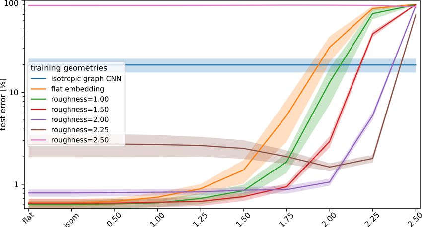
To test the performance on, and generalization between, different geometries, we train equivalent
GEM-CNN models on a flat mesh and meshes with a roughness of 1, 1.5, 2, 2.25 and 2.5. Each
model is tested individually on each of the considered test geometries, which are the flat mesh,
isometric embeddings and curved embeddings with a roughness of 0.5, 1, 1.25, 1.5, 1.75, 2, 2.25
and 2.5. Figure 3 shows the test errors of the GEM-CNNs on the different train geometries (different
curves) for all test geometries (shown on the x-axis). Since our model is purely defined in terms
of the intrinsic geometry of a mesh, it is expected to be insensitive to isometric changes in the
embeddings. This is empirically confirmed by the fact that the test performances on flat and isometric
embeddings are exactly equal. As expected, the test error increases for most models with the surface
roughness. Models trained on more rough surfaces are hereby more robust to deformations. The
models generalize well from a rough training to smooth test geometry up to a training roughness of
1.5. Beyond that point, the test performances on smooth meshes degrades up to the point of random
guessing at a training roughness of 2.5.
As a baseline, we build an isotropic graph CNN with the same network topology and number of
parameters (≈ 163k). This model is insensitive to the mesh geometry and therefore performs exactly
equal on all surfaces. While this enhances its robustness on very rough meshes, its test error of
19.80 ± 3.43% is an extremely bad result on MNIST. In contrast, the use of anisotropic filters of
GEM-CNN allows it to reach a test error of only 0.60 ± 0.05% on the flat geometry. It is therefore
competitive with conventional CNNs on pixel grids, which apply anisotropic kernels as well. More
details on the datasets, models and further experimental setup are given in appendix E.1.
6.2 S HAPE C ORRESPONDENCE
As a second experiment, we perform non-rigid shape correspondence on the FAUST dataset (Bogo
et al., 2014), following Masci et al. (2015) . The data consists of 100 meshes of human bodies in
various positions, split into 80 train and 20 test meshes. The vertices are registered, such that vertices
8Under review as a conference paper at ICLR 2021
Model Features Accuracy (%)
ACNN (Boscaini et al., 2016) SHOT 62.4
Geodesic CNN (Masci et al., 2015) SHOT 65.4
MoNet (Monti et al., 2016) SHOT 73.8
FeaStNet (Verma et al., 2018) XYZ 98.7
ZerNet (Sun et al., 2018) XYZ 96.9
SpiralNet++ (Gong et al., 2019) XYZ 99.8
Graph CNN XYZ 1.40±0.5
Graph CNN SHOT 23.80±8
Non-equiv. CNN (SHOT frames) XYZ 73.00±4.0
Non-equiv. CNN (SHOT frames) SHOT 75.11±2.4
GEM-CNN XYZ 99.73±0.04
GEM-CNN (broken symmetry) XYZ 99.89±0.02
Figure 3: Test errors for MNIST digit classifica-
tion on embedded meshes. Except for the isotropic
graph CNN, different curves correspond to the Table 2: Results of FAUST shape correspondence.
same GEM-CNN model, trained on different train- Statistics are means and standard errors of the mean of
ing geometries. The x-axis shows different test over three runs. All cited results are from their respective
geometries on which each model is tested. Shaded papers.
regions state the standard errors of the means over
6 runs.
on the same position on the body, such as the tip of the left thumb, have the same identifier on all
meshes. All meshes have 6890 vertices, making this a 6890-class segmentation problem.
We use a simple architecture, which transforms the vertices’ XY Z coordinates, which are of type 3ρ0 ,
via 6 convolutional layers to a feature of type 64ρ0 , with intermediate features of type 16(ρ0 ⊕ρ1 ⊕ρ2 ).
The convolutional layers use residual connections and the RegularNonlinearity with N = 5 samples.
Afterwards, we use two 1×1 convolutions with ReLU to map first to 256 channels and finally to 6890
channels, after which a softmax predicts the registration probabilities. The 1×1 convolutions use a
dropout of 50% and 1E-4 weight decay. The network is trained with a cross entropy loss with an
initial learning rate of 0.01, which is halved when training loss reaches a plateau.
As all meshes in the FAUST dataset share the same topology, breaking the gauge equivariance in
higher layers can actually be beneficial. As shown in (Weiler & Cesa, 2019), symmetry can be broken
by treating non-invariant features as invariant features as input to the final 1×1 convolution. Such
architectures are equivariant on lower levels, while allowing orientation sensitivity at higher layers.
As baselines, we compare to various models, some of which use more complicated pipelines, such as
(1) the computation of geodesics over the mesh, which requires solving partial differential equations,
(2) pooling, which requires finding a uniform sub-selection of vertices, (3) the pre-computation of
SHOT features which locally describe the geometry (Tombari et al., 2010), or (4) post-processing
refinement of the predictions. The GEM-CNN requires none of these additional steps. In addition,
we compare to SpiralNet++ (Gong et al., 2019), which requires all inputs to be similarly meshed.
Finally, we compare to an isotropic version of the GEM-CNN, which reduces to a conventional graph
CNN, as well as a non-gauge-equivariant CNN based on SHOT frames. The results in table 2 show
that the GEM-CNN outperforms prior works and a non-gauge-equivariant CNN, that isotropic graph
CNNs are unable to solve the task and that for this data set breaking gauge symmetry in the final
layers of the network is beneficial. More experimental details are given in appendix E.2.
7 C ONCLUSIONS
Convolutions on meshes are commonly performed as a convolution on their underlying graph, by
forgetting geometry, such as orientation of neighbouring vertices. In this paper we propose Gauge
Equivariant Mesh CNNs, which endow Graph Convolutional Networks on meshes with anisotropic
kernels and parallel transport. Hence, they are sensitive to the mesh geometry, and result in equivalent
outputs regardless of the arbitrary choice of kernel orientation.
We demonstrate that the inference of GEM-CNNs is invariant under isometric deformations of
meshes and generalizes well over a range of non-isometric deformations. On the FAUST shape
correspondence task, we show that Gauge equivariance, combined with symmetry breaking in the
final layer, leads to state of the art performance.
9Under review as a conference paper at ICLR 2021
R EFERENCES
Bekkers, E. J., Lafarge, M. W., Veta, M., Eppenhof, K. A., Pluim, J. P., and Duits, R. Roto-translation
covariant convolutional networks for medical image analysis. In International Conference on
Medical Image Computing and Computer-Assisted Intervention (MICCAI), 2018.
Bogo, F., Romero, J., Loper, M., and Black, M. J. Faust: Dataset and evaluation for 3d mesh
registration. In Proceedings of the IEEE Conference on Computer Vision and Pattern Recognition,
pp. 3794–3801, 2014.
Boscaini, D., Masci, J., Rodolà, E., and Bronstein, M. M. Learning shape correspondence with
anisotropic convolutional neural networks. In NIPS, 2016.
Bouritsas, G., Bokhnyak, S., Ploumpis, S., Bronstein, M., and Zafeiriou, S. Neural 3d morphable
models: Spiral convolutional networks for 3d shape representation learning and generation. In
Proceedings of the IEEE International Conference on Computer Vision, pp. 7213–7222, 2019.
Bronstein, M. M., Bruna, J., LeCun, Y., Szlam, A., and Vandergheynst, P. Geometric deep learning:
Going beyond Euclidean data. IEEE Signal Processing Magazine, 2017.
Cohen, T. and Welling, M. Group equivariant convolutional networks. In ICML, 2016.
Cohen, T. S. and Welling, M. Steerable CNNs. In ICLR, 2017.
Cohen, T. S., Geiger, M., and Weiler, M. A general theory of equivariant CNNs on homogeneous
spaces. In Conference on Neural Information Processing Systems (NeurIPS), 2019a.
Cohen, T. S., Weiler, M., Kicanaoglu, B., and Welling, M. Gauge equivariant convolutional networks
and the Icosahedral CNN. 2019b.
Crane, K., Desbrun, M., and Schröder, P. Trivial connections on discrete surfaces. Computer Graphics
Forum (SGP), 29(5):1525–1533, 2010.
Crane, K., de Goes, F., Desbrun, M., and Schröder, P. Digital geometry processing with discrete
exterior calculus. In ACM SIGGRAPH 2013 courses, SIGGRAPH ’13, New York, NY, USA, 2013.
ACM.
Cucurull, G., Wagstyl, K., Casanova, A., Veličković, P., Jakobsen, E., Drozdzal, M., Romero, A.,
Evans, A., and Bengio, Y. Convolutional neural networks for mesh-based parcellation of the
cerebral cortex. 2018.
Defferrard, M., Bresson, X., and Vandergheynst, P. Convolutional neural networks on graphs with fast
localized spectral filtering. In Advances in neural information processing systems, pp. 3844–3852,
2016.
Gallier, J. and Quaintance, J. Differential Geometry and Lie Groups: A Computational Perspective,
volume 12. Springer Nature, 2020.
Gong, S., Chen, L., Bronstein, M., and Zafeiriou, S. Spiralnet++: A fast and highly efficient mesh
convolution operator. In Proceedings of the IEEE International Conference on Computer Vision
Workshops, pp. 0–0, 2019.
Hanocka, R., Fish, N., Wang, Z., Giryes, R., Fleishman, S., and Cohen-Or, D. Alignet: Partial-shape
agnostic alignment via unsupervised learning. ACM Transactions on Graphics (TOG), 38(1):1–14,
2018.
Hoogeboom, E., Peters, J. W. T., Cohen, T. S., and Welling, M. HexaConv. In International
Conference on Learning Representations (ICLR), 2018.
Kipf, T. N. and Welling, M. Semi-Supervised Classification with Graph Convolutional Networks. In
ICLR, 2017.
Kondor, R., Lin, Z., and Trivedi, S. Clebsch-gordan nets: a fully fourier space spherical convolutional
neural network. In NIPS, 2018.
10Under review as a conference paper at ICLR 2021
Lai, Y.-K., Jin, M., Xie, X., He, Y., Palacios, J., Zhang, E., Hu, S.-M., and Gu, X. Metric-driven rosy
field design and remeshing. IEEE Transactions on Visualization and Computer Graphics, 16(1):
95–108, 2009.
Lang, L. and Weiler, M. A Wigner-Eckart Theorem for Group Equivariant Convolution Kernels.
arXiv preprint arXiv:2010.10952, 2020.
Maron, H., Galun, M., Aigerman, N., Trope, M., Dym, N., Yumer, E., Kim, V. G., and Lipman, Y.
Convolutional neural networks on surfaces via seamless toric covers. ACM Trans. Graph., 36(4):
71–1, 2017.
Masci, J., Boscaini, D., Bronstein, M. M., and Vandergheynst, P. Geodesic convolutional neural
networks on riemannian manifolds. ICCVW, 2015.
Monti, F., Boscaini, D., Masci, J., Rodolà, E., Svoboda, J., and Bronstein, M. M. Geometric deep
learning on graphs and manifolds using mixture model cnns. CoRR, abs/1611.08402, 2016. URL
http://arxiv.org/abs/1611.08402.
Perraudin, N., Defferrard, M., Kacprzak, T., and Sgier, R. Deepsphere: Efficient spherical convo-
lutional neural network with healpix sampling for cosmological applications. Astronomy and
Computing, 27:130–146, 2019.
Poulenard, A. and Ovsjanikov, M. Multi-directional geodesic neural networks via equivariant
convolution. ACM Transactions on Graphics, 2018.
Qi, C. R., Su, H., Mo, K., and Guibas, L. J. Pointnet: Deep learning on point sets for 3d classification
and segmentation. In Proceedings of the IEEE conference on computer vision and pattern
recognition, pp. 652–660, 2017a.
Qi, C. R., Yi, L., Su, H., and Guibas, L. J. Pointnet++: Deep hierarchical feature learning on point
sets in a metric space. In Advances in neural information processing systems, pp. 5099–5108,
2017b.
Riegler, G., Osman Ulusoy, A., and Geiger, A. Octnet: Learning deep 3d representations at high
resolutions. In Proceedings of the IEEE Conference on Computer Vision and Pattern Recognition,
pp. 3577–3586, 2017.
Schonsheck, S. C., Dong, B., and Lai, R. Parallel Transport Convolution: A New Tool for Convolu-
tional Neural Networks on Manifolds. arXiv:1805.07857 [cs, math, stat], May 2018.
Serre, J.-P. Linear representations of finite groups. 1977.
Sosnovik, I., Szmaja, M., and Smeulders, A. Scale-equivariant steerable networks. In International
Conference on Learning Representations (ICLR), 2020.
Sun, Z., Rooke, E., Charton, J., He, Y., Lu, J., and Baek, S. Zernet: Convolutional neural networks
on arbitrary surfaces via zernike local tangent space estimation. arXiv preprint arXiv:1812.01082,
2018.
Tchapmi, L., Choy, C., Armeni, I., Gwak, J., and Savarese, S. Segcloud: Semantic segmentation of
3d point clouds. In 2017 international conference on 3D vision (3DV), pp. 537–547. IEEE, 2017.
Thomas, N., Smidt, T., Kearnes, S., Yang, L., Li, L., Kohlhoff, K., and Riley, P. Tensor Field
Networks: Rotation- and Translation-Equivariant Neural Networks for 3D Point Clouds. 2018.
Tombari, F., Salti, S., and Di Stefano, L. Unique signatures of histograms for local surface description.
In European conference on computer vision, pp. 356–369. Springer, 2010.
Tu, L. W. Differential geometry: connections, curvature, and characteristic classes, volume 275.
Springer, 2017.
Verma, N., Boyer, E., and Verbeek, J. Feastnet: Feature-steered graph convolutions for 3d shape
analysis. In Proceedings of the IEEE Conference on Computer Vision and Pattern Recognition, pp.
2598–2606, 2018.
11Under review as a conference paper at ICLR 2021
Weiler, M. and Cesa, G. General E(2)-equivariant steerable CNNs. In Conference on Neural
Information Processing Systems (NeurIPS), 2019. URL https://arxiv.org/abs/1911.
08251.
Weiler, M., Geiger, M., Welling, M., Boomsma, W., and Cohen, T. 3D Steerable CNNs: Learning
Rotationally Equivariant Features in Volumetric Data. In NeurIPS, 2018a.
Weiler, M., Hamprecht, F. A., and Storath, M. Learning steerable filters for rotation equivariant
CNNs. In Conference on Computer Vision and Pattern Recognition (CVPR), 2018b.
Wiersma, R., Eisemann, E., and Hildebrandt, K. CNNs on Surfaces using Rotation-Equivariant
Features. Transactions on Graphics, 39(4), July 2020. doi: 10.1145/3386569.3392437.
Winkels, M. and Cohen, T. S. 3D G-CNNs for pulmonary nodule detection. In Conference on
Medical Imaging with Deep Learning (MIDL), 2018.
Worrall, D. and Welling, M. Deep scale-spaces: Equivariance over scale. In Conference on Neural
Information Processing Systems (NeurIPS), 2019.
Worrall, D. E. and Brostow, G. J. Cubenet: Equivariance to 3D rotation and translation. In European
Conference on Computer Vision (ECCV), 2018.
Worrall, D. E., Garbin, S. J., Turmukhambetov, D., and Brostow, G. J. Harmonic Networks: Deep
Translation and Rotation Equivariance. In CVPR, 2017.
Wu, Z., Song, S., Khosla, A., Yu, F., Zhang, L., Tang, X., and Xiao, J. 3d shapenets: A deep
representation for volumetric shapes. In Proceedings of the IEEE conference on computer vision
and pattern recognition, pp. 1912–1920, 2015.
Zhao, F., Xia, S., Wu, Z., Duan, D., Wang, L., Lin, W., Gilmore, J. H., Shen, D., and Li, G. Spherical
u-net on cortical surfaces: Methods and applications. CoRR, abs/1904.00906, 2019a. URL
http://arxiv.org/abs/1904.00906.
Zhao, Y., Birdal, T., Lenssen, J. E., Menegatti, E., Guibas, L., and Tombari, F. Quaternion equivariant
capsule networks for 3d point clouds. arXiv preprint arXiv:1912.12098, 2019b.
12You can also read