ITERATIVE ENERGY-BASED PROJECTION ON A NOR- MAL DATA MANIFOLD FOR ANOMALY LOCALIZATION
←
→
Page content transcription
If your browser does not render page correctly, please read the page content below
Published as a conference paper at ICLR 2020

I TERATIVEENERGY- BASED PROJECTION ON A NOR -
MAL DATA MANIFOLD FOR ANOMALY LOCALIZATION

 David Dehaene∗, Oriel Frigo∗, Sébastien Combrexelle, Pierre Eline
 AnotherBrain, Paris, France
 {david, oriel, sebastien, pierre}@anotherbrain.ai

                                              A BSTRACT

             Autoencoder reconstructions are widely used for the task of unsupervised anomaly
             localization. Indeed, an autoencoder trained on normal data is expected to only
             be able to reconstruct normal features of the data, allowing the segmentation of
             anomalous pixels in an image via a simple comparison between the image and
             its autoencoder reconstruction. In practice however, local defects added to a nor-
             mal image can deteriorate the whole reconstruction, making this segmentation
             challenging. To tackle the issue, we propose in this paper a new approach for
             projecting anomalous data on a autoencoder-learned normal data manifold, by us-
             ing gradient descent on an energy derived from the autoencoder’s loss function.
             This energy can be augmented with regularization terms that model priors on what
             constitutes the user-defined optimal projection. By iteratively updating the input
             of the autoencoder, we bypass the loss of high-frequency information caused by
             the autoencoder bottleneck. This allows to produce images of higher quality than
             classic reconstructions. Our method achieves state-of-the-art results on various
             anomaly localization datasets. It also shows promising results at an inpainting
             task on the CelebA dataset.

1       I NTRODUCTION
Automating visual inspection on production lines with artificial intelligence has gained popularity
and interest in recent years. Indeed, the analysis of images to segment potential manufacturing
defects seems well suited to computer vision algorithms. However these solutions remain data
hungry and require knowledge transfer from human to machine via image annotations. Furthermore,
the classification in a limited number of user-predefined categories such as non-defective, greasy,
scratched and so on, will not generalize well if a previously unseen defect appears. This is even more
critical on production lines where a defective product is a rare occurrence. For visual inspection, a
better-suited task is unsupervised anomaly detection, in which the segmentation of the defect must
be done only via prior knowledge of non-defective samples, constraining the issue to a two-class
segmentation problem.
From a statistical point of view, an anomaly may be seen as a distribution outlier, or an observation
that deviates so much from other observations as to arouse suspicion that it was generated by a
different mechanism (Hawkins, 1980). In this setting, generative models such as Variational Au-
toEncoders (VAE, Kingma & Welling (2014)), are especially interesting because they are capable
to infer possible sampling mechanisms for a given dataset. The original autoencoder (AE) jointly
learns an encoder model, that compresses input samples into a low dimensional space, and a de-
coder, that decompresses the low dimensional samples into the original input space, by minimizing
the distance between the input of the encoder and the output of the decoder. The more recent variant,
VAE, replaces the deterministic encoder and decoder by stochastic functions, enabling the modeling
of the distribution of the dataset samples as well as the generation of new, unseen samples. In both
models, the output decompressed sample given an input is often called the reconstruction, and is
used as some sort of projection of the input on the support of the normal data distribution, which
we will call the normal manifold. In most unsupervised anomaly detection methods based on VAE,
models are trained on flawless data and defect detection and localization is then performed using a
    ∗
        Equal contributions.

                                                     1
Published as a conference paper at ICLR 2020

distance metric between the input sample and its reconstruction (Bergmann et al., 2018; 2019; An
& Cho, 2015; Baur et al., 2018; Matsubara et al., 2018).
One fundamental issue in this approach is that the models learn on the normal manifold, hence there
is no guarantee of the generalization of their behavior outside this manifold. This is problematic
since it is precisely outside the dataset distribution that such methods intend to use the VAE for
anomaly localization. Even in the case of a model that always generates credible samples from the
dataset distribution, there is no way to ensure that the reconstruction will be connected to the input
sample in any useful way. An example illustrating this limitation is given in figure 1, where a VAE
trained on regular grid images provides a globally poor reconstruction despite a local perturbation,
making the anomaly localization challenging.
In this paper, instead of using the VAE reconstruction, we propose to find a better projection of an
input sample on the normal manifold, by optimizing an energy function defined by an autoencoder
architecture. Starting at the input sample, we iterate gradient descent steps on the input to converge
to an optimum, simultaneously located on the data manifold and closest to the starting input. This
method allows us to add prior knowledge about the expected anomalies via regularization terms,
which is not possible with the raw VAE reconstruction. We show that such an optimum is better than
previously proposed autoencoder reconstructions to localize anomalies on a variety of unsupervised
anomaly localization datasets (Bergmann et al., 2019) and present its inpainting capabilities on the
CelebA dataset (Liu et al., 2015). We also propose a variant of the standard gradient descent that
uses the pixel-wise reconstruction error to speed up the convergence of the energy.

                (a) Training      (b) Anomalous          (c) VAE         (d) Gradient-
                   sample             sample          reconstruction    based projection

Figure 1: Even though an anomaly is a local perturbation in the image (b), the whole VAE-
reconstructed image can be disturbed (c). Our gradient descent-based method gives better quality
reconstructions (d).

2     BACKGROUND

2.1   G ENERATIVE MODELS

In unsupervised anomaly detection, the only data available during training are samples x from a
non-anomalous dataset X ⊂ Rd . In a generative setting, we suppose the existence of a proba-
bility function of density q, having its support on all Rd , from which the dataset was sampled.
The generative objective is then to model an estimate of density q, from which we can obtain
new samples close to the dataset. Popular generative architectures are Generative Adversarial Net-
works (GAN, Goodfellow et al. (2014)), that concurrently train a generator G to generate sam-
ples from random, low-dimensional noise z ∼ p, z ∈ Rl , l  d, and a discriminator D to
classify generated samples and dataset samples. This model converges to the equilibrium of the
expectation over both real and generated datasets of the binary cross entropy loss of the classifier
minG maxD [ Ex∼q [log(D(x))] + Ez∼p [log(1 − D(G(z)))] ].
Disadvantages of GANs are that they are notoriously difficult to train (Goodfellow, 2017), and they
suffer from mode collapse, meaning that they have the tendency to only generate a subset of the
original dataset. This can be problematic for anomaly detection, in which we do not want some
subset of the normal data to be considered as anomalous (Bergmann et al., 2019). Recent works
such as Thanh-Tung et al. (2019) offer simple and attractive explanations for GAN behavior and
propose substantial upgrades, however Ravuri & Vinyals (2019) still support the point that GANs
have more trouble than other generative models to cover the whole distribution support.

                                                  2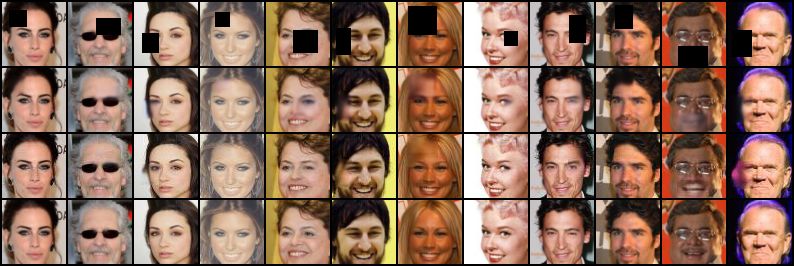
Published as a conference paper at ICLR 2020

Another generative model is the VAE (Kingma & Welling (2014)), where, similar to a GAN genera-
tor, a decoder model tries to approximate the dataset distribution with a simple latent variables prior
p(z), with z ∈R Rl , and conditional distributions output by the decoder p(x|z). This leads to the esti-
mate p(x) = p(x|z)p(z)dz, that we would like to optimize using maximum likelihood estimation
on the dataset. To render the learning tractable with a stochastic gradient descent (SGD) estimator
with reasonable variance, we use importance sampling, introducing density functions q(z|x) output
by an encoder network, and Jensen’s inequality to get the variational lower bound :

                                           p(x|z)p(z)
                 log p(x) = log Ez∼q(z|x)
                                             q(z|x)                                                 (1)
                           ≥ Ez∼q(z|x) log p(x|z) − DKL (q(z|x)kp(z)) = −L(x)

We will use L(x) as our loss function for training. We define the VAE reconstruction, per anal-
ogy with an autoencoder reconstruction, as the deterministic sample fV AE (x) that we obtain by
encoding x, decoding the mean of the encoded distribution q(z|x), and taking again the mean of the
decoded distribution p(x|z).
VAEs are known to produce blurry reconstructions and generations, but Dai & Wipf (2019) show
that a huge enhancement in image quality can be gained by learning the variance of the decoded
distribution p(x|z). This comes at the cost of the distribution of latent variables produced by the
encoder q(z) being farther away from the prior p(z), so that samples generated by sampling z ∼
p(z), x ∼ p(x|z) have poorer quality. The authors show that using a second VAE learned on samples
from q(z), and sampling from it with ancestral sampling u ∼ p(u), z ∼ p(z|u), x ∼ p(x|z), allows
to recover samples of GAN-like quality. The original autoencoder can be roughly considered as a
VAE whose encoded and decoded distributions have infinitely small variances.

2.2   A NOMALY DETECTION AND LOCALIZATION

We will consider that an anomaly is a sample with low probability under our estimation of the
dataset distribution. The VAE loss, being a lower bound on the density, is a good proxy to clas-
sify samples between the anomalous and non-anomalous categories. To this effect, a threshold
T can be defined on the loss function, delimiting anomalous samples with L(x) ≥ T and nor-
mal samples L(x) < T . However, according to Matsubara et al. (2018), the regularization term
LKL (x) = DKL (q(z|x)kp(z)) has a negative influence in the computation of anomaly scores. They
propose instead an unregularized score Lr (x) = −Ez∼q(z|x) log p(x|z) which is equivalent to the
reconstruction term of a standard autoencoder and claim a better anomaly detection.
Going from anomaly detection to anomaly localization, this reconstruction term becomes crucial to
most of existing solutions. Indeed, the inability of the model to reconstruct a given part of an image
is used as a way to segment the anomaly, using a pixel-wise threshold on the reconstruction error.
Actually, this segmentation is very often given by a pixel-wise (An & Cho, 2015; Baur et al., 2018;
Matsubara et al., 2018) or patch-wise comparison of the input image, and some generated image,
as in Bergmann et al. (2018; 2019), where the structural dissimilarity (DSSIM, Wang et al. (2004))
between the input and its VAE reconstruction is used.
Autoencoder-based methods thus provide a straightforward way of generating an image conditioned
on the input image. In the GAN original framework, though, images are generated from random
noise z ∼ p(z) and are not conditioned by an input. Schlegl et al. (2017) propose with AnoGAN to
get the closest generated image to the input using gradient descent on z for an energy defined by:

                     EAnoGAN = ||x − G(z)||1 + λ · ||fD (x) − fD (G(z))||1                          (2)

The first term ensures that the generation G(z) is close to the input x. The second term is based
on a distance between features of the input and the generated images, where fD (x) is the output of
an intermediate layer of the discriminator. This term ensures that the generated image stays in the
vicinity of the original dataset distribution.

                                                   3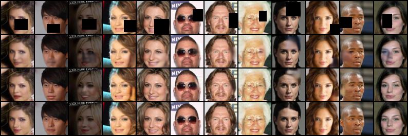
Published as a conference paper at ICLR 2020

Figure 2: Illustration of our method. We perform gradient descent on E(xt ) to iteratively correct
xt .

3     P ROPOSED METHOD
3.1   A DVERSARIAL PROJECTIONS

According to Zimmerer et al. (2018), the loss gradient with respect to x gives the direction towards
normal data samples, and its magnitude could indicate how abnormal a sample is. In their work on
anomaly identification, they use the loss gradient as an anomaly score.
Here we propose to use the gradient of the loss to iteratively improve the observed x. We propose
to link this method to the methodology of computing adversarial samples in Szegedy et al. (2014).
After training a VAE on non-anomalous data, we can define a threshold T on the reconstruction loss
Lr as in (Matsubara et al., 2018), such that a small proportion of the most improbable samples are
identified as anomalies. We obtain a binary classifier defined by

                                                1 if Lr (x) ≥ T
                                    A(x) =                                                     (3)
                                                0 otherwise

Our method consists in computing adversarial samples of this classifier (Szegedy et al., 2014), that
is to say, starting from a sample x0 with A(x0 ) = 1, iterate gradient descent steps over the input x,
constructing samples x1 , . . . xN , to minimize the energy E(x), defined as
                                 E(xt ) = Lr (xt ) + λ · ||xt − x0 ||1                              (4)

An iteration is done by calculating xt+1 as
                                     xt+1 = xt − α · ∇x E(xt ),                                     (5)

where α is a learning rate parameter, and λ is a parameter trading off the inclusion of xt in the
normal manifold, given by Lr (xt ), and the proximity between xt and the input x0 , assured by the
regularization term ||xt − x0 ||1 .

3.2   R EGULARIZATION TERM

We model the anomalous images that we encounter as normal images in which a region or several
regions of pixels are altered but the rest of the pixels are left untouched. To recover the best segmen-
tation of the anomalous pixels from an anomalous image xa , we want to recover the closest image
from the normal manifold xg . The term closest has to be understood in the sense that the smallest
number of pixels are modified between xa and xg . In our model, we therefore would like to use the
L0 distance as a regularization distance of the energy. Since the L0 distance is not differentiable, we
use the L1 distance as an approximation.

3.3   O PTIMIZATION IN INPUT SPACE

While in our method the optimization is done in the input space, in the previously mentioned
AnoGAN, the search for the optimal reconstruction is done by iterating over z samples with the

                                                   4
Published as a conference paper at ICLR 2020
energy defined in equation 2. Following the aforementioned analogy between a GAN generator G
and a VAE decoder Dec, a similar approach in the context of a VAE would be to use the energy
||x − Dec(z)||1 − λ · log p(z) (6)
where the − log p(z) term has the same role as AnoGAN’s ||fD (x) − fD (G(z))||1 term, to ensure
that Dec(z) stays within the learned manifold. We chose not to iterate over z in the latent space
for two reasons. First, because as noted in Dai & Wipf (2019) and Hoffman & Johnson (2016), the
prior p(z) is not always a good proxy for the real image of the distribution in the latent space q(z).
Second, because the VAE tends to ignore some details of the original image in its reconstruction,
considering that these details are part of the independent pixel noise allowed by the modeling of
p(x|z) as a diagonal Gaussian, which causes its infamous blurriness. An optimization in latent
space would have to recreate the high frequency structure of the image, whereas iterating over the
input image space, and starting the descent on the input image x0 , allows us to keep that structure
and thus to obtain projections of higher quality.
3.4 O PTIMIZING GRADIENT DESCENT
We observed that using the Adam optimizer (Kingma & Ba, 2015) is beneficial for the quality of the
optimization. Moreover, to speed up the convergence and further preserve the aforementioned high
frequency structure of the input, we propose to compute our iterative samples using the pixel-wise
reconstruction error of the VAE. To explain the intuition behind this improvement, we will consider
the inpainting task. In this setting, as in anomaly localization, a local perturbation is added on top of
a normal image. However, in the classic inpainting task, the localization of the perturbation is known
beforehand, and we can use the localization mask Ω to only change the value of the anomalous pixels
in the gradient descent:
xt+1 = xt − α · ( ∇x E(xt ) Ω) (7)
where is the Hadamard product.
For anomaly localization and blind inpainting, where this information is not available, we compute
the pixel-wise reconstruction error which gives a rough estimate of the mask. The term ∇x E(xt ) is
therefore replaced with ∇x E(xt ) (xt − fV AE (xt ))2 ) in equation 5:
xt+1 = xt − α · ( ∇x E(xt ) (xt − fV AE (xt ))2 ) (8)
where fV AE (x) is the standard reconstruction of the VAE. Optimizing the energy this way, a pixel
where the reconstruction error is high will update faster, whereas a pixel with good reconstruction
will not change easily. This prevents the image to update its pixels where the reconstruction is
already good, even with a high learning rate. As can be seen in appendix B, this method converges
to the same performance as the method of equation 5, but with fewer iterations. An illustration of
our method can be found in figure 2.
3.5 S TOP CRITERION
A standard stop criterion based on the convergence of the energy can efficiently be used. Using
the adversarial setting introduced in section 3.1, we also propose to stop the gradient descent when
a certain predefined threshold on the VAE loss is reached. For example, such a threshold can be
chosen to be a quantile of the empirical loss distribution computed on the training set.
4 E XPERIMENTS
In this section, we evaluate the proposed method for two different applications: anomaly segmen-
tation and image inpainting. Both applications are interesting use cases of our method, where we
search to reconstruct partially corrupted images, correcting the anomalies while preserving the un-
corrupted image regions.
4.1 U NSUPERVISED ANOMALY SEGMENTATION
In order to evaluate the proposed method for the task of anomaly segmentation, we perform experi-
ments with the recently proposed MVTec dataset (Bergmann et al., 2019). This collection of datasets
5Published as a conference paper at ICLR 2020
Table 1: Results for anomaly segmentation on MVTec datasets, expressed in AUROC (Area Un-
der the Receiver Operating Characteristics). Four different baselines are trained on normal samples
and are augmented by our proposed gradient based reconstruction (grad) for comparison: A deter-
ministic autoencoder trained with L2 loss (L2 AE) as in (Bergmann et al., 2019); A deterministic
autoencoder trained with DSSIM loss (DSAE) as in (Bergmann et al., 2019); A variational autoen-
coder (VAE); And a variational autoencoder with a learned decoder variance (γ-VAE) as in (Dai &
Wipf, 2019). For each result a green or red background denotes respectively an improvement or a
decrease in performance compared to the baseline. It can be seen that the proposed gradient-based
reconstruction achieves the best segmentation for most datasets, with a mean improvement rate of
9.52% over all baselines.
L2 AE DSAE VAE γ-VAE
Category L2 AE DSAE VAE γ-VAE
grad grad grad grad
carpet 0.539 0.734 0.545 0.774 0.580 0.735 0.648 0.727
Textures
grid 0.960 0.981 0.960 0.980 0.888 0.961 0.950 0.979
leather 0.751 0.921 0.710 0.602 0.834 0.925 0.818 0.897
tile 0.476 0.575 0.496 0.626 0.465 0.654 0.491 0.581
wood 0.630 0.805 0.641 0.738 0.695 0.838 0.665 0.809
bottle 0.909 0.916 0.933 0.951 0.902 0.922 0.913 0.931
cable 0.732 0.864 0.790 0.859 0.828 0.910 0.777 0.880
capsule 0.786 0.952 0.769 0.884 0.862 0.917 0.814 0.917
hazelnut 0.976 0.984 0.966 0.966 0.977 0.976 0.977 0.988
Objects
metalnut 0.880 0.899 0.881 0.920 0.881 0.907 0.883 0.914
pill 0.885 0.912 0.895 0.927 0.888 0.930 0.897 0.935
screw 0.979 0.980 0.983 0.925 0.958 0.945 0.976 0.972
toothbrush 0.971 0.983 0.973 0.984 0.971 0.985 0.971 0.983
transistor 0.906 0.921 0.904 0.934 0.894 0.919 0.896 0.931
zipper 0.680 0.889 0.828 0.887 0.814 0.869 0.706 0.871
consists of 15 different categories of objects and textures in the context of industrial inspection, each
category containing a number of normal and anomalous samples.
We train our model on normal training samples and test it on both normal and anomalous test sam-
ples to evaluate the anomaly segmentation performance.
We perform experiments with three different baseline autoencoders: A “vanilla” variational autoen-
coder with decoder covariance matrix fixed to identity (Kingma & Welling, 2014), a variational
autoencoder with learned decoder variance (Dai & Wipf, 2019), a “vanilla” deterministic autoen-
coder trained with L2 as reconstruction loss (L2 AE) and a deterministic autoencoder trained with
DSSIM reconstruction loss (DSAE), as proposed by Bergmann et al. (2018). For the sake of a fair
comparison, all the autoencoder models are parameterized by convolutional neural networks with the
same architecture, latent space dimensionality (set to 100), learning rate (set to 0.0001) and number
of epochs (set to 300). The architecture details (layers, paddings, strides) are the same as described
in Bergmann et al. (2018) and Bergmann et al. (2019). Similarly to the authors in Bergmann et al.
(2019), for the textures datasets, we first subsample the original dataset images to 512 × 512 and
then crop random patches of size 128 × 128 which are used to train and test the different models.
For the object datasets, we directly subsample the original dataset images to 128 × 128 unlike in
Bergmann et al. (2019) who work on 256 × 256 images, then we perform rotation and translation
data augmentations. For all datasets we train on 10000 images.
Anomaly segmentation is then computed by reconstructing the anomalous image and comparing it
with the original. We perform the comparison between reconstructed and original with the DSSIM
metric as it has been observed in Bergmann et al. (2018) that it provides better anomaly localization
than L2 or L1 distances. For the gradient descent, we set the step size α := 0.5, L1 regularization
weight λ := 0.05 and the stop criterion is achieved when a sample reconstruction loss is inferior to
the minimum reconstruction loss over the training set.
In table 1 we show the AUROC (Area Under the Receiver Operating Characteristics) for different
autoencoder methods, with different thresholds applied to the DSSIM anomaly map computed be-
6Published as a conference paper at ICLR 2020
tween original and reconstructed images. Note that an AUROC of 1 expresses the best possible
segmentation in terms of normal and anomalous pixels. For each autoencoder variant we compare
the baseline reconstruction with the proposed gradient-based reconstruction (grad.). As in Bergmann
et al. (2019) we observe that an overall best model is hard to identify, however we show that our
method increases the AUC values for almost all autoencoder variants. Aggregating the results over
all datasets and baselines, we report a mean improvement rate of 9.52%, with a median of 4.33%, a
25th percentile of 1.86%, and a 75th percentile of 15.86%. The histogram of the improvement rate
for all datasets and baselines is provided in appendix F, as well as a short analysis.
In figure 3 we compare our anomaly segmentation with a baseline L2 autoencoder Bergmann et al.
(2019) (L2 AE) for a number of image categories. For all results in figure 3, we set the same threshold
to 0.2 to the anomaly detection map given by the DSSIM metric. The visual results in figure 3
highlights an overall improvement of anomaly localization by our proposed iterative reconstruction
(L2 AE-grad). See appendix C for additional visual results of anomaly segmentation on remaining
categories of MVTec dataset, and on remaining baseline models.
Normal
Anomalous
L2 AE
L2 AE-grad
Figure 3: First row: Normal samples of hazelnut, grid, cable, wood, carpet and bottle categories in
MVTec dataset; Second row: anomalous samples from the aforementioned dataset categories; Third
row: Anomaly segmentation with baseline L2 autoencoder (Bergmann et al., 2019); Fourth row:
our proposed anomaly segmentation with L2 autoencoder augmented with gradient-based iterative
reconstruction. Ground truth is represented by red contour, and each estimated segmentation by a
green overlay. It can be seen that anomaly segmentation is refined by our proposed method, with a
tendency of detecting less false positives.
4.2 I NPAINTING
Image inpainting is a well known image reconstruction problem which consists of reconstructing a
corrupted or missing part of an image, where the region to be reconstructed is usually given by a
known mask. Many different approaches for inpainting have been proposed in the literature, such
as anisotropic diffusion (Bertalmio et al., 2000), patch matching (Criminisi et al., 2004), context
autoencoders (Pathak et al., 2016) and conditional variational autoencoders (Ivanov et al., 2019).
If we consider that the region to be reconstructed is not known beforehand, the problem is sometimes
called blind inpainting (Altinel et al., 2018), and the corrupted part can be seen as an anomaly to be
corrected.
7Published as a conference paper at ICLR 2020
(a) Masked (b) Blind (c) Inpaint, (d) Blind (e) Inpaint, (f) Ground
images inpaint, VAE VAE inpaint, ours ours truth
Figure 4: Inpainting experiment performed on CelebA dataset, where the test face images are
masked with uniform noise. The baseline VAE reconstruction is disturbed by the noise mask, pro-
viding a poor inpainting. The proposed gradient-based VAE provides a more convincing inpainting
by an iterative process.
We performed experiments with image inpainting on the CelebA dataset (Liu et al., 2015), which
consists of celebrity faces. In figure 4 we compare the inpainting results obtained with a baseline
VAE with learned variance (γ-VAE) and Resnet architecture, as described by Dai & Wipf (2019),
with the same VAE model, augmented by our proposed gradient-based iterative reconstruction. Note
that for the regular inpainting task, gradients are multiplied by the inpainting mask at each iteration
(equation 7), while for the blind inpainting task, the mask is unknown. See appendix D for a com-
parison with a recent method based on variational autoencoders, proposed by Ivanov et al. (2019).
5 R ELATED W ORK
Baur et al. (2018) have used autoencoder reconstructions to localize anomalies in MRI scans, and
have compared several variants using diverse per-pixel distances as well as perceptual metrics de-
rived from a GAN-like architecture. Bergmann et al. (2018) use the structural similarity metric
(Wang et al., 2004) to compare the original image and its reconstruction to achieve better anomaly
localization, and also presents the SSIM autoencoder, which is trained directly with this metric.
Zimmerer et al. (2018) use the derivative of the VAE loss function with respect to the input, called
the score. The amplitude of the score is supposed to indicate how abnormal a pixel is. While we
agree that the gradient of the loss is an indication of an anomaly, we think that we have to integrate
this gradient over the path from the input to the normal manifold to obtain meaningful information.
We compare our results to score-based results for anomaly localization in appendix A.
The work that is the most related to ours is AnoGAN (Schlegl et al., 2017). We have mentioned
above the differences between the two approaches, which, apart from the change in underlying ar-
chitectures, boil down to the ability in our method to update directly the input image instead of
searching for the optimal latent code. This enables the method to converge faster and above all to
keep higher-frequency structures of the input, which would have been deteriorated if it were passed
through the AE bottleneck. Bergmann et al. (2019) compare standard AE reconstructions tech-
niques to AnoGAN, and observes that AnoGAN’s performances on anomaly localizations tasks are
poorer than AE’s due to the mode collapse tendency of GAN architectures. Interestingly, updates on
AnoGAN such as fast AnoGAN (Schlegl et al., 2019) or AnoVAEGAN (Baur et al., 2018) replaced
the gradient descent search of the optimal z with a learned encoder model, yielding an approach
very similar to the standard VAE reconstruction-based approaches, but with a reconstruction loss
learned by a discriminator, which is still prone to mode collapse (Thanh-Tung et al., 2019).
8Published as a conference paper at ICLR 2020
6 C ONCLUSION
In this paper, we proposed a novel method for unsupervised anomaly localization, using gradient
descent of an energy defined by an autoencoder reconstruction loss. Starting from a sample under
test, we iteratively update this sample to reduce its autoencoder reconstruction error. This method
offers a way to incorporate human priors into what is the optimal projection of an out-of-distribution
sample into the normal data manifold. In particular, we use the pixel-wise reconstruction error to
modulate the gradient descent, which gives impressive anomaly localization results in only a few
iterations. Using gradient descent in the input data space, starting from the input sample, enables us
to overcome the autoencoder tendency to provide blurry reconstructions and keep normal high fre-
quency structures. This significantly reduces the number of pixels that could be wrongly classified
as defects when the autoencoder fails to reconstruct high frequencies. We showed that this method,
which can easily be added to any previously trained autoencoder architecture, gives state-of-the-art
results on a variety of unsupervised anomaly localization datasets, as well as qualitative reconstruc-
tions on an inpainting task. Future work can focus on replacing the L1 -based regularization term
with a Bayesian prior modeling common types of anomalies, and on further improving the speed of
the gradient descent.
R EFERENCES
Fazil Altinel, Mete Ozay, and Takayuki Okatani. Deep structured energy-based image inpainting.
In 2018 24th International Conference on Pattern Recognition (ICPR), pp. 423–428, Aug 2018.
doi: 10.1109/ICPR.2018.8546025.
Jinwon An and Sungzoon Cho. Variational autoencoder based anomaly detection using reconstruc-
tion probability. Technical report, SNU Data Mining Center, 2015.
Christoph Baur, Benedikt Wiestler, Shadi Albarqouni, and Nassir Navab. Deep autoencoding models
for unsupervised anomaly segmentation in brain MR images. CoRR, abs/1804.04488, 2018.
Paul Bergmann, Sindy Löwe, Michael Fauser, David Sattlegger, and Carsten Steger. Improv-
ing unsupervised defect segmentation by applying structural similarity to autoencoders. CoRR,
abs/1807.02011, 2018.
Paul Bergmann, Michael Fauser, David Sattlegger, and Carsten Steger. Mvtec ad — a comprehensive
real-world dataset for unsupervised anomaly detection. CVPR, 2019.
Marcelo Bertalmio, Guillermo Sapiro, Vincent Caselles, and Coloma Ballester. Image inpainting. In
Proceedings of the 27th Annual Conference on Computer Graphics and Interactive Techniques,
SIGGRAPH ’00, pp. 417–424, New York, NY, USA, 2000. ACM Press/Addison-Wesley Publish-
ing Co. ISBN 1-58113-208-5. doi: 10.1145/344779.344972.
Antonio Criminisi, Patrick Pérez, and Kentaro Toyama. Region filling and object removal by
exemplar-based image inpainting. Trans. Img. Proc., 13(9):1200–1212, September 2004. ISSN
1057-7149. doi: 10.1109/TIP.2004.833105.
Bin Dai and David P. Wipf. Diagnosing and enhancing VAE models. CoRR, abs/1903.05789, 2019.
Ian Goodfellow, Jean Pouget-Abadie, Mehdi Mirza, Bing Xu, David Warde-Farley, Sherjil Ozair,
Aaron Courville, and Yoshua Bengio. Generative adversarial nets. In Advances in neural infor-
mation processing systems, pp. 2672–2680, 2014.
Ian J. Goodfellow. NIPS 2016 tutorial: Generative adversarial networks. CoRR, abs/1701.00160,
2017.
Douglas M Hawkins. Identification of outliers. Monographs on applied probability and statistics.
Chapman and Hall, London [u.a.], 1980. ISBN 041221900X.
Matthew D. Hoffman and Matthew J. Johnson. Elbo surgery: yet another way to carve up the
variational evidence lower bound. In NIPS 2016 Workshop on Advances in Approximate Bayesian
Inference, 2016.
9Published as a conference paper at ICLR 2020
Oleg Ivanov, Michael Figurnov, and Dmitry Vetrov. Variational autoencoder with arbitrary condi-
tioning. In International Conference on Learning Representations, 2019.
Diederik P. Kingma and Jimmy Ba. Adam: A method for stochastic optimization. In Yoshua Bengio
and Yann LeCun (eds.), 3rd International Conference on Learning Representations, ICLR 2015,
San Diego, CA, USA, May 7-9, 2015, Conference Track Proceedings, 2015.
Diederik P. Kingma and Max Welling. Auto-encoding variational bayes. In Yoshua Bengio and Yann
LeCun (eds.), 2nd International Conference on Learning Representations, ICLR 2014, Banff, AB,
Canada, April 14-16, 2014, Conference Track Proceedings, 2014.
Ziwei Liu, Ping Luo, Xiaogang Wang, and Xiaoou Tang. Deep learning face attributes in the wild.
In Proceedings of International Conference on Computer Vision (ICCV), December 2015.
Takashi Matsubara, Ryosuke Tachibana, and Kuniaki Uehara. Anomaly machine component detec-
tion by deep generative model with unregularized score. CoRR, abs/1807.05800, 2018.
Deepak Pathak, Philipp Krähenbühl, Jeff Donahue, Trevor Darrell, and Alexei Efros. Context en-
coders: Feature learning by inpainting. In Computer Vision and Pattern Recognition (CVPR),
2016.
Suman V. Ravuri and Oriol Vinyals. Classification accuracy score for conditional generative models.
CoRR, abs/1905.10887, 2019.
Thomas Schlegl, Philipp Seeböck, Sebastian M Waldstein, Ursula Schmidt-Erfurth, and Georg
Langs. Unsupervised anomaly detection with generative adversarial networks to guide marker
discovery. In International Conference on Information Processing in Medical Imaging, pp. 146–
157. Springer, 2017.
Thomas Schlegl, Philipp Seeböck, Sebastian M. Waldstein, Georg Langs, and Ursula Schmidt-
Erfurth. f-anogan: Fast unsupervised anomaly detection with generative adversarial networks.
Medical Image Analysis, 54:30 – 44, 2019. ISSN 1361-8415. doi: https://doi.org/10.1016/j.
media.2019.01.010.
Christian Szegedy, Wojciech Zaremba, Ilya Sutskever, Joan Bruna, Dumitru Erhan, Ian J. Good-
fellow, and Rob Fergus. Intriguing properties of neural networks. In Yoshua Bengio and Yann
LeCun (eds.), 2nd International Conference on Learning Representations, ICLR 2014, Banff, AB,
Canada, April 14-16, 2014, Conference Track Proceedings, 2014.
Hoang Thanh-Tung, Truyen Tran, and Svetha Venkatesh. Improving generalization and stability of
generative adversarial networks. CoRR, abs/1902.03984, 2019.
Zhou Wang, Alan Bovik, Hamid Sheikh, and Eero Simoncelli. Image quality assessment: From
error visibility to structural similarity. Image Processing, IEEE Transactions on, 13:600 – 612,
05 2004. doi: 10.1109/TIP.2003.819861.
David Zimmerer, Jens Petersen, Simon A. A. Kohl, and Klaus H. Maier-Hein. A case for the score:
Identifying image anomalies using variational autoencoder gradients. In 32nd Conference on
Neural Information Processing Systems (NeurIPS 2018), 2018.
David Zimmerer, Fabian Isensee, Jens Petersen, Simon Kohl A. A., and Klaus H. Maier-Hein. Un-
supervised anomaly localization using variational auto-encoders. CoRR, abs/1907.02796, 2019.
10Published as a conference paper at ICLR 2020
A C OMPARISON WITH Z IMMERER ET AL . (2019)
Table 2: Complementary results for anomaly segmentation on MVTec datasets, expressed in AU-
ROC for different pixel-wise scores derived from a baseline VAE: from left to right, squared error
reconstruction ||x − fV AE (x)||2 (denoted Lr (x)), gradient of the loss |∇x L(x)|, combination of
both, gradient of the KL divergence |DKL (q(z|x)kp(z)) (denoted |∇x LKL (x)|) as well as combi-
nation of KL derivative and error reconstruction as suggested in Zimmerer et al. (2018; 2019).
|∇x L(x)| |∇x LKL (x)|
Category Lr (x) |∇x L(x)| |∇x LKL (x)| VAE-grad
Lr (x) Lr (x)
carpet 0.537 0.580 0.566 0.553 0.555 0.735
Textures
grid 0.823 0.635 0.812 0.507 0.790 0.961
leather 0.783 0.650 0.792 0.627 0.791 0.925
tile 0.547 0.606 0.581 0.623 0.588 0.654
wood 0.686 0.691 0.726 0.643 0.713 0.838
bottle 0.831 0.762 0.832 0.629 0.830 0.922
cable 0.831 0.796 0.846 0.674 0.841 0.910
capsule 0.765 0.754 0.772 0.642 0.795 0.917.
hazelnut 0.907 0.831 0.908 0.468 0.885 0.976
Objects
metalnut 0.833 0.831 0.870 0.710 0.834 0.907
pill 0.869 0.833 0.872 0.480 0.826 0.930
screw 0.851 0.726 0.842 0.412 0.795 0.945
toothbrush 0.942 0.798 0.943 0.619 0.939 0.985
transistor 0.788 0.843 0.834 0.801 0.836 0.919
zipper 0.725 0.674 0.729 0.562 0.727 0.869
Zimmerer et al. (2019) proposed to perform anomaly localization using different scores derived
from the gradient of the VAE loss. In particular, it has been shown that the product of the VAE
reconstruction error with the gradient of the KL divergence was very informative for medical images.
In table 2 we compare the pixel-wise anomaly detection AUROC of these different scores with our
method. For all experiments, we use the same “vanilla” VAE as described in section 4.1.
It can be seen that other VAE-based methods using a single evaluation of the gradient are constantly
outperformed by our method.
11Published as a conference paper at ICLR 2020
B C ONVERGENCE SPEED
Figure 5: Evolution of pixel-wise anomaly detection AUROC performance.
In figure 5 we compare the number of iterations needed to reach convergence with our two proposals
for gradient descent: Standard update as in equation 5 and Tuned update using a gradient mask
computed with the VAE reconstruction error, as in equation 8. The model is a VAE with learned
decoder variance (Dai & Wipf, 2019), trained on the Grid dataset (Bergmann et al., 2019). We
compute the mean pixel-wise anomaly detection AUROC after each iteration on the test set.
We can see that the tuned method converges to the same performance as the standard method, with
far fewer iterations.
12Published as a conference paper at ICLR 2020
C A DDITIONAL ANOMALY SEGMENTATION RESULTS
Figure 6: From left to right: Normal; Anomalous; Anomaly segmentation with baseline L2 autoen-
coder (Bergmann et al., 2019); Our proposed anomaly segmentation with L2 autoencoder augmented
with gradient-based iterative reconstruction.
13Published as a conference paper at ICLR 2020
L2 AE
L2 AE-grad
DSAE
DSAE-grad
VAE
VAE-grad
γ-VAE
γ-VAE-grad
Figure 7: Illustration of anomaly localization comparison over four baselines (L2 AE, DSAE, VAE,
γ-VAE). Ground truth is represented by red contour, and each estimated segmentation by a green
overlay. It can be seen that anomaly segmentation is overall improved when different baselines are
augmented by our proposed gradient descent.
14Published as a conference paper at ICLR 2020
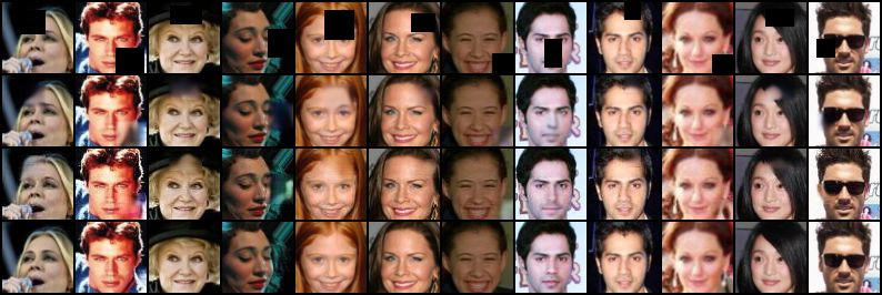
D I NPAINTING COMPARISON
Figure 8: Inpainting comparison. Each batch is made of four rows, from top to bottom: Masked
input image; VAE with arbitrary conditioning (VAEAC, Ivanov et al. (2019)); Ours; Ground truth.
The quality of the reconstructions is comparable, even though our VAE is trained without any as-
sumptions over the mask’s properties.
15Published as a conference paper at ICLR 2020
E I LLUSTRATION OF THE OPTIMIZATION PROCESS
Figure 9: Principle of the energy optimization to project anomalous sample on the normal manifold
Figure 9 illustrates our method principle. We start with a defective input x0 whose reconstruction
x̂0 does not necessarily lie on the normal data manifold. As the optimization process carries on, the
optimized sample x0 and its reconstruction look more similar and get closer to the manifold. The
regularization term of the energy function makes sure that the optimized sample stays close to the
original sample.
16Published as a conference paper at ICLR 2020
F D ISTRIBUTION OF THE IMPROVEMENT RATE ON MVT EC AD
Figure 10: Distribution of the improvement rate over all presented baselines and all datasets in
MVTec AD.
Figure 10 shows the distribution of the AUC improvement rate over all presented baselines and all
datasets in MVTec AD using our gradient-based projection method.
AU Cgrad − AU Cbase
improvement rate =
AU Cbase
• 8.3% of data points are under the 0 value delimiting an increase or decrease in AUC due to
our method, and 91.7% data points are over this value. Our method increases the AUC in a
vast majority of cases.
• The median is at 4.33%, the 25th percentile at 1.86%, and the 75th percentile at 15.86%.
17You can also read