Scholarship@Western Western University
←
→
Page content transcription
If your browser does not render page correctly, please read the page content below
Western University
Scholarship@Western

Bone and Joint Institute

9-1-2020

Application of a novel automatic method for determining the
bilateral symmetry midline of the facial skeleton based on
invariant moments
Rodrigo Dalvit Carvalho da Silva
Western University

Thomas Richard Jenkyn
Western University

Victor Alexander Carranza
Western University

Follow this and additional works at: https://ir.lib.uwo.ca/boneandjointpub

   Part of the Medicine and Health Sciences Commons

Citation of this paper:
da Silva, Rodrigo Dalvit Carvalho; Jenkyn, Thomas Richard; and Carranza, Victor Alexander, "Application of
a novel automatic method for determining the bilateral symmetry midline of the facial skeleton based on
invariant moments" (2020). Bone and Joint Institute. 614.
https://ir.lib.uwo.ca/boneandjointpub/614
!"#!$%&'(!
SS symmetry                                                                                      !"#$%&'

Article
Application of a Novel Automatic Method for
Determining the Bilateral Symmetry Midline of the
Facial Skeleton Based on Invariant Moments
Rodrigo Dalvit Carvalho da Silva 1,2, *, Thomas Richard Jenkyn 1,2,3,4,5 and
Victor Alexander Carranza 1,6
 1   Craniofacial Injury and Concussion Research Laboratory, Western University,
     London, ON N6A 3K7, Canada; tjenkyn@uwo.ca (T.R.J.); vcarranz@uwo.ca (V.A.C.)
 2   School of Biomedical Engineering, Faculty of Engineering, Western University,
     London, ON N6A 3K7, Canada
 3   Department of Mechanical and Materials Engineering, Western University, London, ON N6A 3K7, Canada
 4   School of Kinesiology, Faculty of Health Sciences, Western University, London, ON N6A 3K7, Canada
 5   Wolf Orthopaedic Biomechanics Laboratory, Fowler Kennedy Sport Medicine Clinic,
     London, ON N6A 3K7, Canada
 6   School of Biomedical Engineering, Faculty of Engineering, Collaborative Specialization in Musculoskeletal
     Health Research, and Bone and Joint Institue, Western University, London, ON N6A 3K7, Canada
 *   Correspondence: rdalvitc@uwo.ca
                                                                                                      !"#!$%&'(!
 Received: 17 August 2020; Accepted: 1 September 2020; Published: 3 September 2020                    !"#$%&'

 Abstract: Assuming a symmetric pattern plays a fundamental role in the diagnosis and surgical
 treatment of facial asymmetry, for reconstructive craniofacial surgery, knowing the precise location of
 the facial midline is important since for most reconstructive procedures the intact side of the face
 serves as a template for the malformed side. However, the location of the midline is still a subjective
 procedure, despite its importance. This study aimed to automatically locate the bilateral symmetry
 midline of the facial skeleton based on an invariant moment technique using pseudo-Zernike
 moments. A total of 367 skull images were evaluated using the proposed technique. The technique
 was found to be reliable and provided good accuracy in the symmetry planes. This new technique
 will be utilized for subsequent studies to evaluate diverse craniofacial reconstruction techniques.

 Keywords: craniofacial skeleton; cephalometric analysis; pseudo-Zernike moments; independent
 component analysis; principal component analysis; k-nearest neighbours

1. Introduction
      Bilateral symmetry refers to a structure of interest having two sides, with one side being the
mirror image of the other. A good example is the human skull, which has bilateral symmetry of its
left and right sides. The goal of reconstructive surgery for clinical pathologies of the craniofacial
skeleton, whether boney deformities, mandibular alterations, tumors, or trauma, is to restore bilateral
symmetry in order to restore function. Similarly, clinical diagnosis and treatment for orthodontics [1],
maxillofacial [2], cosmetic [3], and plastic reconstructive surgery [4] seek to restore craniofacial bilateral
symmetry. In preceding studies, a method for finding the midline of the craniofacial skeleton was
developed by the authors of [5]. This is now a generally accepted method for establishing the
midline of the face. However, accurately locating the craniofacial midline is essential for correctly
forming an intact template for correcting facial malformations or trauma and for the planning of
procedures in the reconstruction process. To date, the most common method for locating the midline
for a two-dimensional image, or the midsagittal plane (MSP) for a three-dimensional object, has been
the method proposed by the authors of [6].

Symmetry 2020, 12, 1448; doi:10.3390/sym12091448                              www.mdpi.com/journal/symmetry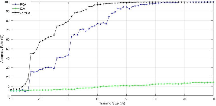
Symmetry 2020, 12, 1448                                                                           2 of 13

      Midline symmetry planes have been calculated as a perpendicular midpoint for a stack of
horizontal lines crossing bilaterally across the facial skeleton containing boney landmarks or by
using boney landmarks to construct a midline that best represents facial symmetry [7]. A simple way
to define the midline has been to manually select a number of cephalometric boney landmarks
in the dataset, either directly on the plane or at equal distances on either side of the midline
plane. However, this requires great attention and care during the selection process by an expert
user. Manual selection of skeletal landmarks is time-consuming and unreliable, which results in
less accurate estimations of symmetry. In addition, the results have been dependent on the user’s
ability to find appropriate landmarks, the landmark availability and the visibility of the anatomical
landmarks [8].
      Methods with some amount of automation have been attempted for finding the midline plane.
The authors of [9] described a semi-automatic approach for calculating the symmetry plane of the facial
skeleton using principal component analysis (PCA) and the iterative closest point (ICP) alignment
method along with surface models reconstructed from computed tomography image data. The initial
step was to determine the precise position of the mirror plane using PCA in order to approximately
align the mirrored mesh and the original mesh. The ICP algorithm was then used to get a refined
registration [10]. The disadvantage of this method was the need for a central point of the image for
the calculation of the symmetric plane. This point was obtained using the average of the vertices
of the facial mesh. If this point was not provided or if the point was in wrong location, in case of
imperfect symmetry, this method could lead to an error in the construction of the symmetric plane.
A second limitation lied in the lack of self-learning or the ability to learn. Once applied to an image,
the subsequent image will not learn or improve its performance based on the previous data.
      Most recently, an upgraded version of a mirroring and registration technique for automatic
symmetry plane detection of 3D asymmetrically scanned human faces was discussed in [11]. This work
described an ICP-based method that uses particle swarm optimization. This method starts from
a 3D discrete model and evaluates the symmetry plane by a preliminary first-attempt, carried
out with a PCA algorithm, which is then refined iteratively until its final estimation obtained by
a Levenberg–Marquardt algorithm. This new proposed method was claimed to improve upon the
limitations from the authors’ previous algorithm [12]; however, the new model still has limitations
and fails to incorporate self-learning to improve the model’s outcome. For instance, in the case of
craniofacial dysmorphism, this model requires the user to interactively segment the area to solve the
asymmetry. However, if the algorithm is presented a similar image again, another intervention is
required to select the area.
      The aim of this study was to present a technique for the automatic calculation of the craniofacial
symmetry midline using invariant moments. Figure 1 shows the steps of the proposed algorithm.
First, based on the cephalometric landmarks, the image is rotated so that the midline passes through
the center, i.e., 0 . The image is then duplicated and a dataset of 30 images of 1 resolution is created
from 14 to 15 . This set of images is then passed through different feature extractors and then to
the k-nearest neighbors classifier. In the classification phase, pseudo-Zernike moments (PZMs) and
PCA were selected after going through the independent component analysis (ICA) feature extractor.
A second set of images of 0.5 degrees resolution was taken from the centered images to test the PZMs
and PCA. PZMs were selected for having achieved the best accuracy. After the classifier determines
the rotation degree of these images, their midpoints are found. Finally, by joining the midpoints and
grades described by the classifier, the midlines can be constructed.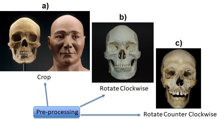
Symmetry 2020, 12, 1448                                                                                3 of 13

                                  Figure 1. Steps of the proposed method.

2. Materials and Methods

2.1. Image Creation
      To create the dataset, the IdentifyMe database [13] was used. This database contains 464 skull
images composed of skull and digital face images (real-world examples of solved skull identification
cases) and unlabeled supplementary skull images. The database also contains several unsuitable
images that needed to be corrected before being added to the dataset. Additionally, this step intended
to eliminate regions of non-interest through cropping and the correction of image rotation so that the
processing efficiency of the system could be enhanced (Figure 2).

     Figure 2. An example of images in the IdentifyMe database that required pre-processing in which the
     image was (a) cropped, (b) rotated clockwise, and (c) rotated counter clockwise.

     As the cropping process can be easily solved, the focus was to create a method to correct the
rotation, since it will be necessary for training purpose. The first step was to manually identify six
cephalometric landmarks (1-Crista Galli, 2-Frontozygomatic Suture, 3-Orbitale, 4-Anterior Nasal Spine,
5-Subspinale, and 6-Prosthion) (Figure 3a). Then, using a grid as reference, the images were rotated
using the nearest neighbor interpolation technique so that landmarks 1, 4, 5, and 6 were vertically
aligned and landmarks 2 and 3 were horizontally aligned with their respective counterpart as in
Figure 3b. These images were used as a gold standard to create the rotated images.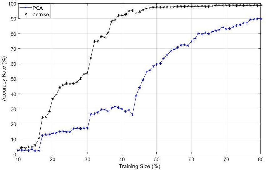
Symmetry 2020, 12, 1448 4 of 13
Figure 3. Pre-processing step to vertically align images. (a) The six cephalometric landmarks are
identified. (b) A grid is then added to the image and rotated so that the landmarks can be horizontally
and vertically aligned.
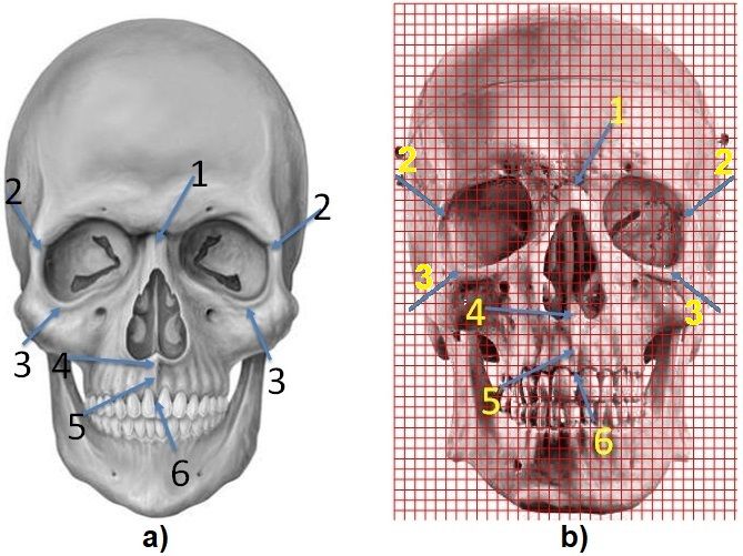
After the images were vertically aligned, 367 images were selected as suitable for use. Based on
each image, 30 images were created with inclination angles from 14 to 15 degrees with 1 degree
of variation along the sagittal plane, totaling 11,010 images (Figure 4). Those angles were also used
as the image labels in the classification step. Finally, the images were resized to 128 ⇥ 128 using
the nearest neighbor interpolation method. A resolution of 128 ⇥ 128 was selected so as to reduce
the processing time and computational energy during the creation of PCA and ICA feature vectors.
Due to the limitations of the i7-8850H CPU (2.60 GHz) with 16 GB RAM computer used, a resolution
of 256 ⇥ 256 resulted in the computer crashing.
Figure 4. The unrotated image (original) was labeled as “0” and subsequent images were labelled
based on the angle of rotation.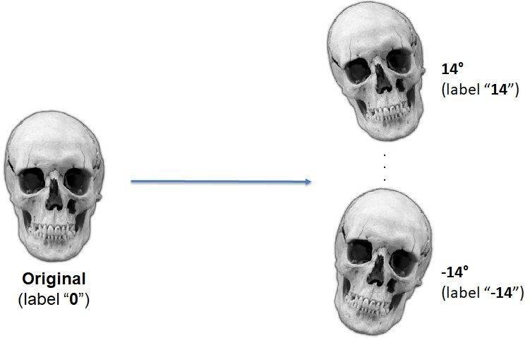
Symmetry 2020, 12, 1448                                                                          5 of 13

2.2. Feature Extractors
    Three feature extraction methods (PZMs, ICA, and PCA) were compared to determine the method
with the leading accuracy. The resultant method was then used for the algorithm to determine the
midpoint to generate the final midlines.

2.2.1. Pseudo-Zernike Moments-PZMs
      Zernike moments (ZMs) were first introduced in computer vision by the authors of [14] and
are widely used to identify and highlight global features of an image in image processing and
machine learning applications [15]. Zernike moments map an image into a set of complex Zernike
polynomials. As these Zernike polynomials are orthogonal to each other, Zernike moments can
represent the properties of an image without redundancy or overlap of information between moments.
Pseudo-Zernike moments are a derivation of the Zernike moments that was shown to be more robust
and less sensitive to image noise [16].
      Pseudo-Zernike moments, i.e., pseudo-Zernike polynomials, are one of the best invariant image
descriptors belonging to a family of circularly orthogonal moments due to their minimal information
redundancy, robustness to image noise, provision of twice the number of moments, and having more
low-order moments. In addition to being rotational invariants, they can be made into scale and
translation invariants after certain geometric transformations. PZMs have been used in numerous
machine learning and image analysis applications, such as cephalometric landmark detection [17],
Alzheimer’s disease detection ([18–20]), medical image retrieval [21], detection of tumors and brain
tumors ([22–24]), facial expression [25] and facial age recognition [26], facial recognition ([27,28]),
and other industrial applications [29].
      As described by the authors of [15], to calculate the PZMs, the image (or region of interest) is
initially mapped into a unit disc, where the center of the image is the origin of the disc (Figure 5a).
Pixels that are outside the disc are not used in the calculation. To include these pixels (Figure 5b)
the disc can be expanded so that the image function f(x,y) is completely enclosed inside the disc by
performing the following:
                              p      p                        p      p
                                2      2                       2         2
                    xi =          +      x,     and    yj =                      y,                 (1)
                               2    N 1                       2     N        1

where x = y = 0, 1, ... (N 1), xi , and y j are the image coordinates, and the image function f(x,y) is
defined over the discrete square domain N ⇥ N.

                           Figure 5. (a) Image mapped over and (b) enclosed in a unit disc.
Symmetry 2020, 12, 1448 6 of 13
Obtaining the PZMs [15] of an image begins with the calculation of the pseudo-Zernike
polynomials (PZP) Vpq (xi ,y j ) of order p and repetition q:
Vpq (xi ,y j ) = R pq (r)e jqq , (2)
q
where p is a non-negative integer, 0 |q| p, q = tan 1 ( y/x ), q 2 [0,2p], and r = xi2 + y2j .
The complex function Vpq (xi ,y j ) has two separate parts: the radial polynomials R pq (r) and the angular
functions e jqq = (cosq + j sinq )q polynomials in cosq and sinq. The radial polynomials are expressed as:
p |q|
(2p + 1 s)!r p s
R pq (r) = Â ( 1) s . (3)
s =0
s!( p+ | q | +1 s)!( p | q | s)!
Since R pq (r) = R p, q (r), we consider q 0 and rewrite Equation (3) as:
p
R pq (r) = Â Bpqs rs , (4)
s=q
where
( 1) p s ( p + s + 1) !
B pqs = . (5)
( p s ) ! ( s + q + 1) ! ( s q ) !
A p-recursive method focusing on reducing time complexity through the fast computing of the
pseudo-Zernike radial polynomials using a hybrid method was presented by the authors of [30],
where:
Rqq (r ) = r q , (6)
R(q+1)q (r ) = (2q + 3)r q+1 2( q + 1)r q , (7)
R pq (r ) = (k1 r + k2 ) R( p 1) q ( r ) + k 3 R ( p 2) q ( r ),
(8)
p = q + 2, q + 3, ..., pmax ,
where
2p(2p + 1)
k1 = , (9)
( p + q + 1)( p q)
( p + q)( p q 1)
k2 = 2p + k1 , (10)
(2p 1)
(p + q 1)( p q 2)
k3 = (2p 1)( p 1) k 1 + 2( p 1) k 2 . (11)
2
The PZMs of order p and repetition q of an image function f(xi ,y j ) over a unit disc are represented
in a discrete domain by:
N 1N 1
p+1
A pq =
p   ⇤
f ( xi , y j )Vpq ( xi , y j )Dxi Dy j . (12)
i =0 j =0Symmetry 2020, 12, 1448 7 of 13
2.2.2. Independent Component Analysis—ICA
ICA is a blind source separation or statistical signal processing technique where a given
measurement is represented by a linear composition of statistically independent components (ICs) that
aims to linearly decompose a random vector into components that are as independent as possible [31].
Given a set of random variables {x1 (t), x2 (t), ..., xn (t)}, where t is time or the sample index, it is
assumed to be generated as a linear mixture of ICs {s1 (t), s2 (t), ..., sn (t)}:
x = ( x1 (t), x2 (t), ..., xn (t)) T = A(s1 (t), s2 (t), ..., sn (t)) T = As, (13)
where A is an unknown mixture matrix A Rn⇥n . The FastICA algorithm [31] was used to perform the
task through the columns of its mixture matrix, which contain the main feature vectors.
2.2.3. Principal Component Analysis—PCA
PCA, first introduced by the authors of [32] and then independently developed by the authors
of [33], is a technique that preserves the variation present in a large number of interrelated variables of
a dataset while reducing the dimensionality. This is achieved by transforming the dataset into a new
ordered set of uncorrelated variables or principal components (PCs), so that all the original variables
can be represented by the first few variables that maintained the most important features [34].
2.3. Geometric Moments—Central Point
In current applications, the central point of the face is obtained manually. Thus, we propose
the application of the geometric moments method for the automatic extraction of the central point.
Geometric moments are a popular method of moments and have been used to identify the image
centroid in a number of image processing tasks [35,36].
Two-dimensional (p + q)th order moments of a digitally sampled N ⇥ M image that has the gray
function f ( x, y), ( x, y = 0, ...M 1) [37] is given as:
M pq = Â Â x p yq f ( x, y),
x y (14)
p, q = 0, 1, 2, 3, ... .
As described in [38], the mass and area of the zeroth order moment, M00 , of a digital image is
defined as:
M00 = Â Â f ( x, y). (15)
x y
The center of mass of the image f(x,y) is represented by the two first moments:
M10 = Â Â x f ( x, y), (16)
x y
M01 = Â Â y f ( x, y). (17)
x y
Thus, the centroid of an image can be calculated by:
M10 M01
x̄ = , and ȳ = . (18)
M00 M00Symmetry 2020, 12, 1448 8 of 13
As best practice, the center of mass was chosen to represent the position of an image in the field
of view. The centroid of the image f(x,y), given by Equation (18), can be used to describe the position of
the image in space by using the point as a reference point.
3. Results and Discussions
3.1. Classification
PZMs feature vectors were generated through the first 20 PZM orders and repetitions, based on
Equations (1)–(12), totalizing 121 features. After several tests, the 24 best features were selected to
represent PZMs.
Before being presented to the ICA and PCA feature extractors, the images were vectorized.
For ICA, the mixing matrix A, described in Equation (13), was used as its feature vectors. For PCA,
the eigenvectors based on eigenvalue order on the covariance matrix or its principal components were
used. In total, feature vectors of size 35 were used to represent ICA and PCA.
To make a reasonable comparison among the descriptors, the feature vectors were presented
uniquely to the k-nearest neighbors classifier (k-NN) using the Euclidean distance and the eight nearest
neighbors. In order to evaluate the performance of the feature extractors, the size of the training sets
was varied from 10% to 80% of the available database and the rest was used for testing purposes.
The k-NN outputs were the predicted images angles and Figure 6 presents the comparison of the
accuracy rate among ICA, PCA, and PZMs. Accuracy was calculated using the following model:
CorrectPredictions TP + TN
Accuracy = = , (19)
TotalPredictions TP + TN + FP + FN
where TP—true positives, TN—true negatives, FP—false positives, and FN—false negatives.
Figure 6. Classification accuracy for different feature descriptors, using k-NN and Euclidean distance
for images rotated from 14 to 15 with a resolution of 1 .
The extractor based on the ICA obtained a low accuracy rate with a maximum accuracy of 14.5%
after training, making it unviable for this application. Thus, a further comparison could be carried out
with PZMs versus PCA only to evaluate and finally select the best feature extractor.
Using the selected 367 images and the same inclination angles ( 14 to 15 ), a new set of 59 images
from the original images was created with a 0.5 degree resolution, totaling 21,653 images, and the
results are presented in Figure 7. From these results it can be seen that:
1. PCA performed well, but it required more coefficients to achieve a performance similar to
pseudo-Zernike moments (Figures 6 and 7);Symmetry 2020, 12, 1448 9 of 13
2. In Figure 6, ICA estimation achieved a bad performance in the experiment. We attributed
this to the fact that it is inherently affected by the rotation of the images, which has been already
explored [39];
3. In Figures 6 and 7, pseudo-Zernike moments outperformed ICA and PCA, as PZMs maintained
almost all of the images’ features in a few coefficients.
Figure 7. Classification accuracy for different feature descriptors, using k-NN and Euclidean distance
for images rotated from 14 to 15 with a resolution of 0.5 .
An initial conclusion is that the rotation invariant feature descriptors in the image plane can be
effectively developed using the pseudo-Zernike moments method, which has performed well in these
scenarios. Thus, the superiority and choice of the feature extraction based on pseudo-Zernike moments
in this application became obvious.
3.2. Midpoint Calculation
By using Equations (15)–(18), the center of the image was calculated. To validate the accuracy
of the midpoint technique, visual correctness was used compared with the cephalometric landmarks.
However, a calculation of the image center may be performed manually and compared with
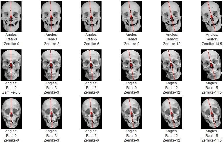
the midpoint. Figure 8 shows three images with rotations of 0 , 3 , 6 , 9 , 12 , and 15 with
centers (midpoints) represented by red stars and the angle directions obtained in the process of
classifying by the pseudo-Zernike moments represented by black dots. To calculate the PZMs,
the 21,653 imagesdataset (obtained from a 0.5 degree resolution) was divided into 80% for training
and 20% for testing, with a total of 4331 testing images. The PZMs method’s accuracy was 98.64%,
and 1.36% of the images received wrong labels (59 images). The images with wrong labels obtained
an error of 0.5 for 33 images, 1 and 1.5 for four images each, 2 , 2.5 , 10 , 13.5 , 14 , and 15 for one
image each, 3.5 for three images, and 3 for two images.
Once the midpoints (red stars) and the angles predicted by k-NN based on PZMs (black dots)
were calculated (Figure 8), the symmetrical line could be easily constructed.Symmetry 2020, 12, 1448 10 of 13
Figure 8. Center of the images calculated using the moment technique. The symmetrical line is
constructed by connecting the midpoint (red star) to the PZMs results (black dots).
The proposed technique presented good results in obtaining the bilateral symmetry midline of
the images. However, there are a few limitations to the proposed technique. A small deviation
in obtaining the center line could be seen in 59 images. This error is likely due to the fact
that some images suffer from a small rotation in the sagittal plane. Additionally, if the images
suffer from deformation, incompleteness, or non-uniform brightness, the image center calculus
becomes difficult to perform since the moment is a quantitative measure of the function or shape
of an image. Furthermore, the algorithm was not tested on non-symmetrical skull images due to a
lack of non-symmetrical skull datasets. Our lab will be collecting non-symmetrical skull images to
test the algorithm further. Another limitation for the proposed method is the resolution size of the
images (128 ⇥ 128). This resolution was selected as any resolution higher than this resulted in an
error from the PC (not enough memory). A higher resolution may result in more accurate results.
However, using the lower resolution of 128 ⇥ 128 created acceptable results.
From the viewpoint of the angles, PZMs performed with 98.64% accuracy in the angles and
1.36% (59 images) with wrong angles. However, 33 of the images (55.93%) had an error of only 0.5 .
The majority of this error could be found in 0.5 , 0 , and 0.5 , where 14 images (42.42% of the
33 images related to 0.5 ) had an error of 0.5 .
It is possible to state that the required resolution of 0.5 reduces the accuracy of the feature
extractor, and this error can be related to the image size, which was resized to improve the processing
of the image matrices. However, these errors can be disregarded as they would be imperceptible to the
human eye.
4. Conclusions
This study proposed an automatic technique for determining the bilateral symmetry midline
of the facial skeleton based on invariant moments. A total of 367 skull images were evaluated
after preprocessing using the IdentifyMe database. A comparative study between pseudo-Zernike
moments, independent component analysis, and principal component analysis as feature descriptors of
images using k-nearest neighbors and Euclidean distance was performed and the study of the feature
extraction step revealed that pseudo-Zernike moments for feature description had the best performance.
PZMs offer an alternative to conventional landmark-based symmetry scores that depends on the
general positions of cephalometric landmarks. PZMs are also an alternative to PCA-ICP techniques,Symmetry 2020, 12, 1448 11 of 13
which depend on the manual selection of the central point and cannot be improved. With the proposed
technique, the central point could be found as the centroid of an image, and then the symmetrical
midline could be constructed.
In this study, we have shown the proposed technique to be reliable and to provide the
midline symmetry plane with great accuracy, which can be used to aid surgeons in reconstructive
craniofacial surgeries.
Author Contributions: Conceptualization, R.D.C.d.S.; Project administration, T.R.J.; Writing—review and editing,
V.A.C. All authors have read and agreed to the published version of the manuscript.
Funding: This research received no external funding.
Conflicts of Interest: The authors declare no conflict of interest.
Disclosure Statement: This study does not contain any experiment with human participants performed by any
of the authors.
References
1. Jiang, X.; Zhang, Y.; Bai, S.; Chang, X.; Wu, L.; Ding, Y. Threedimensional analysis of craniofacial asymmetry
and integrated, modular organization of human head. Int. J. Clin. Exp. Med. 2017, 101, 1424–11431.
2. Romanet, I.; Graillon, N.; Roux, M.K.L.; Guyot, L.; Chossegros, C.; Boutray, M.D.; Foletti, J.M. Hooliganism
and maxillofacial trauma: The surgeon should be warned. J. Stomatol. Oral Maxillofac. Surg. 2019,
120, 106–109. [CrossRef] [PubMed]
3. Guyot, L.; Saint-Pierre, F.; Bellot-Samson, V.; Chikhani, L.; Garmi, R.; Haen, P.; Jammet, P.; Meningaud, J.P.;
Savant, J.; Thomassin, J.M.; et al. Facial surgery for cosmeti purposes: Practice guidelines. J. Stomatol. Oral
Maxillofac. Surg. 2019, 120, 122–127. [CrossRef] [PubMed]
4. Martini, M.; Klausing, A.; Junger, M.; Luchters, G. The self-defining axis of symmetry: A new method to determine
optimal symmetry and its application and limitation in craniofacial surgery. J. Cranio-Maxillo-Fac. Surg. 2017,
45, 1558–1565. [CrossRef]
5. Damstra, J.; Fourie, Z.; De Wit, M. A three-dimensional comparison of a morphometric and conventional
cephalometric midsagittal planes for craniofacial asymmetry. Clin. Oral Investig. 2012, 16, 285–294. [CrossRef]
6. Kim, T.; Baik, J.; Park, J.; Chae, H.; Huh, K. Determination of midsagittal plane for evaluation of facial
asymmetry using three-dimensional computer tomography. Imaging Sci. Dent. 2011, 41, 79–84. [CrossRef]
7. Roumeliotis, G.; Willing, R.; Neuert, M.; Ahluwali, R.; Jenkyn, T.; Yazdani, A. Application of a novel
semi-automatic technique for determining the bilateral symmetry plane of the facial skeleton of normal
adult males. J. Craniofac. Surg. 2015, 26, 1997–2001. [CrossRef]
8. De Momi, E.; Chapuis, J.; pappas, I.; Ferrigno, G.; Hallermann, W.; Schramm, A.; Caversaccio, M. Automatic
extraction of the mid-facial plane for cranio-maxillofacial surgery planning. Int. J. Oral Maxillofac. Surg.
2006, 35, 636–642. [CrossRef]
9. Willing, R.; Roumeliotis, G.; Jenkyn, T.; Yazdani, A. Development and evaluation of a semi-automatic
technique for determining the bilateral symmetry plane of the facial skeleton. Med. Eng. Phys. 2013,
35, 1843–1849. [CrossRef]
10. Zhang, L.; Razdan, A.; Farin, G.; Femiani, J.; Bae, M.; Lockwood, C. 3d face authentication and recognition
based on bilateral symmetry analysis. Vis. Comput. 2006, 22, 43–55. [CrossRef]
11. Angelo, L.D.; Stefano, P.D.; Governi, L.; Marzola, A.; Volpe, Y. A robust and automatic method for the best
symmetry plane detection of craniofacial skeletons. Symmetry 2019, 11, 245. [CrossRef]
12. Angelo, L.D.; Stefano, P.D. A Computational Method for Bilateral Symmetry Recognition in Asymmetrically
Scanned Human Faces. Comput.-Aided Des. Appl. 2014, 11, 275–283. [CrossRef]
13. Nagpal, S.; Singh, M.; Jain, A.; Singh, R.; Vatsa, M.; Noore, A. On Matching Skulls to Digital Face Images:
A Preliminary Approach. CoRR abs/1710.02866. arXiv 2017, arXiv:1710.02866. Available online: http:
//arxiv.org/abs/1710.02866 (accessed on 1 August 2018).
14. Teague, M. Image analysis via the general theory of moments. J. Opt. Soc. Am. 1980, 70, 920–930. [CrossRef]
15. Singh, C.; Walia, E.; Pooja, U.R. Analysis of algorithms for fast computation of pseudo zernike moments and
their numerical stability. Digit. Signal Process. 2012, 22, 1031–1043. [CrossRef]Symmetry 2020, 12, 1448 12 of 13
16. Chee-Way, C.; raveendran, P.; Ramakrishnan, M. An effcient algorithm for fast computation of
pseudo-zernike moments. Int. J. Pattern Recognit. Artif. Intell. 2011, 17. [CrossRef]
17. Kaur, A.; Singh, C. Automatic cephalometric landmark detection using zernike moments and template
matching. Signal Image Video Process. 2013, 9, 117–132. [CrossRef]
18. Shams-Baboli, A.; Ezoji, M. A zernike moment based method for classification of alzheimer’s disease from
structural mri. In Proceedings of the 3rd International Conference on Pattern Recognition and Image Analysis
Faro, Portugal, 20–23 June 2017; pp. 38–43. [CrossRef]
19. Prashar, A. Detection of alzheimer disease using zernike moments. Int. J. Sci. Eng. Res. 2017, 8, 1789–1793.
20. Wang, S.; Du, S.; Zhang, Y.; Phillips, P.; Wu, L.; Chen, X.; Zhang, Y. Alzheimer’s disease detection by
pseudo-zernike moment and linear regression classification. CNS Neurol. Disord. Drug Targets 2017, 16, 11–15.
[CrossRef]
21. Jyothi, B.; Latha, M.; Mohan, P.; Reddy, V. Medical image retrieval using moments. Int. J. Appl. Innov.
Eng. Manag. 2013, 2, 195–200. [CrossRef]
22. Iscan, Z.; Dokur, Z.; Olmez, T. Tumor detection by using zernike moments on segmented magnetic resonance
brain images. Expert Syst. Appl. 2010, 37, 2540–2549. [CrossRef]
23. Thapaliya, K.; Kwon, G. Identification and extraction of brain tumor from mri using local statistics of zernike
moments. Int. J. Imaging Syst. Technol. 2014, 24, 284–292. [CrossRef]
24. Nallasivan, G.; Janakiraman, S. Detection and classification of brain tumors as benign and malignant using
mri scan images and zernike moment feature set with som. J. Comp. Sci. 2016, 10, 24–36.
25. Akkoca, B.; Gökmen, M. Facial expression recognition using local zernike moments. In Proceedings of the
21st Signal Processing and Communications Applications Conference, Haspolat, Turkey, 24–26 April 2013;
pp. 1–4. [CrossRef]
26. Malek, M.; Azimifar, Z.; Boostani, R. Facial age estimation using zernike moments and multi-layer
perception. In Proceedings of the 22nd International Conference on Digital Signal Processing, London, UK,
23–25 August 2017; pp. 1–5. [CrossRef]
27. Rathika, N.; Suresh, P.; Sakthieswaran, N. Face recognition using zernike moments with illumination
variations. Int. J. Biomed. Eng. Technol. 2017, 25, 267–281. [CrossRef]
28. Basaran, E.; Gokmen, M.; Kamasak, M. An efficient multiscale scheme using local zernike moments for face
recognition. Appl. Sci. 2018, 8, 827. [CrossRef]
29. Silva, R.D.C.; Thé, G.A.P.; de Medeiros, F.N.S. Geometrical and statistical feature extraction of images for
rotation invariant classification systems based on industrial devices. In Proceedings of the 21st International
Conference on Automation and Computing (ICAC), Glasgow, UK, 11–12 September 2015; pp. 1–6. [CrossRef]
30. Al-Rawi, M.S. Fast computation of pseudo zernike moments. J. Real-Time Image Process. 2010, 8, 3–10.
[CrossRef]
31. Hyvarinen, A.; Karhunen, J.; Oja, E. Independent Component Analysis; John Wiley and Sons, Inc.: Hoboken, NJ,
USA, 2001. [CrossRef]
32. Pearson, K. On lines and planes of closest fit to systems of points in space. Lond. Edinb. Dublin Philos. Mag.
J. Sci. 1901, 2, 559–572. [CrossRef]
33. Hotelling, H. Analysis of a complex of statistical variables into principal components. J. Educ. Psychol. 1933,
24, 417–441. [CrossRef]
34. Jolliffe, I. Principal Component Analysis, 2nd ed.; Springer: New York, NY, USA, 2002.
35. Zhao, Y.; Ni, R.; Zhu, Z. RST transforms resistant image watermarking based on centroid and sector-shaped
partition. Sci. China Inform. Sci. 2012, 55, 650–662. [CrossRef]
36. Rocha, L.; Velho, L.; Carvalho, P. Image moments-based structuring and tracking of objects. In Proceedings
of the XV Brazilian Symposium on Computer Graphics and Image Processing, Fortaleza Ce, Brazil,
7–10 October 2002; pp. 99–105. [CrossRef]
37. Mercimek, M.; Gulez, K.; Mumcu, T.V. Real object recognition using moment invariants. Sadhana
2005, 30, 765–775. [CrossRef]Symmetry 2020, 12, 1448 13 of 13
38. Xu, D.; Li, H. Geometric Moments Invariants. Pattern Recognit. 2008, 41, 240–249. [CrossRef]
39. Silva, R.D.C.; Thé, G.A.P.; de Medeiros, F.N.S. Rotation-invariant image description from independent
component analysis for classification purposes. In Proceedings of the 12th International Conference on
Informatics in Control, Automation and Robotics (ICINCO), Colmar, France, 21–23 July 2015; pp. 210–216.
c 2020 by the authors. Licensee MDPI, Basel, Switzerland. This article is an open access
article distributed under the terms and conditions of the Creative Commons Attribution
(CC BY) license (http://creativecommons.org/licenses/by/4.0/).You can also read