Neural Network Based Contact Force Control Algorithm for Walking Robots - MDPI
←
→
Page content transcription
If your browser does not render page correctly, please read the page content below
sensors
Letter
Neural Network Based Contact Force Control Algorithm for
Walking Robots
Byeongjin Kim and Soohyun Kim *

                                           Department of Mechanical Engineering, KAIST, Daejeon 34141, Korea; geniuskpj@kaist.ac.kr
                                           * Correspondence: soohyun@kaist.ac.kr

                                           Abstract: Walking algorithms using push-off improve moving efficiency and disturbance rejection
                                           performance. However, the algorithm based on classical contact force control requires an exact model
                                           or a Force/Torque sensor. This paper proposes a novel contact force control algorithm based on
                                           neural networks. The proposed model is adapted to a linear quadratic regulator for position control
                                           and balance. The results demonstrate that this neural network-based model can accurately generate
                                           force and effectively reduce errors without requiring a sensor. The effectiveness of the algorithm is
                                           assessed with the realistic test model. Compared to the Jacobian-based calculation, our algorithm
                                           significantly improves the accuracy of the force control. One step simulation was used to analyze the
                                           robustness of the algorithm. In summary, this walking control algorithm generates a push-off force
                                           with precision and enables it to reject disturbance rapidly.

                                           Keywords: neural network; push-off; walking; force control; contact force; ground reaction force

                                           1. Introduction
                                                 Zero Moment Point (ZMP) control is widely accepted as a basic approach for walking
                                           robots [1–10]. Kajita [11] suggested a preview control system based on the Cart–Table model

                                    to generate biped walking patterns by ZMP. The preview control model requires the Center
                                           of Mass (CoM)’s height and weight to predict a stable CoM trajectory with the desired
Citation: Kim, B.; Kim, S. Neural
                                           ZMP. However, the preview controller is not the most ideal for feedback because ZMP
Network Based Contact Force Control
Algorithm for Walking Robot. Sensors
                                           contains acceleration terms and also real-time feedback control in the influence of external
2021, 21, 287. https://doi.org/
                                           disturbances is challenging. As described in Figure 1a, a ZMP-controlled robot swings its
10.3390/s21010287                          leg in order to take off and touches the leg down softly to the pre-defined footstep placement.
                                           When accelerating, a ZMP-controlled robot only uses its stance leg to accelerate, whereas
Received: 8 December 2020                  humans utilize the propulsive push-off power from the swinging leg to accelerate [12,13]
Accepted: 28 December 2020                 as shown in Figure 1b. The reason why the push-off mechanism is not used for ZMP-
Published: 4 January 2021                  controlled robots is because push-off makes ZMP perturbation. Ground Reaction Forces
                                           (GRFs) from push-off are considered a disturbance, which is one of potential reasons for
Publisher’s Note: MDPI stays neu-          the efficiency gap between humans and robots [14–17]. Therefore, here we propose a new
tral with regard to jurisdictional clai-   control method by push-off that does not cause ZMP perturbation [18].
ms in published maps and institutio-             Atrias [19,20] is a bipedal walking robot co-developed by Carnegie Mellon University
nal affiliations.                          and Oregon State University. The developers of Atrias have shown that Series Elastic
                                           Actuator (SEA) and Spring Loaded Inverted Pendulum (SLIP) model could improve the
                                           efficiency of walking. Atrias achieved a 9 km/h speed and robust walking on an uneven
Copyright: © 2021 by the authors. Li-
                                           terrain with human like GRF. However, because GRF is controlled directly by the SLIP
censee MDPI, Basel, Switzerland.
                                           model, Atrias cannot stand still without making constant motion. Therefore, this solution
This article is an open access article
                                           is not applicable for robots that need to operate at a standstill. The researchers of Atrias
distributed under the terms and con-       calculated a required joint torque using the Jacobian method without using mass terms
ditions of the Creative Commons At-        of foot.
tribution (CC BY) license (https://              A more complicated model does not guarantee a better performance because the
creativecommons.org/licenses/by/           uncertainties are coming from the model. Lee [21] used a null space method to regulate
4.0/).                                     the GRF and kept the robot’s balance. The null space method could control effectively

Sensors 2021, 21, 287. https://doi.org/10.3390/s21010287                                                    https://www.mdpi.com/journal/sensors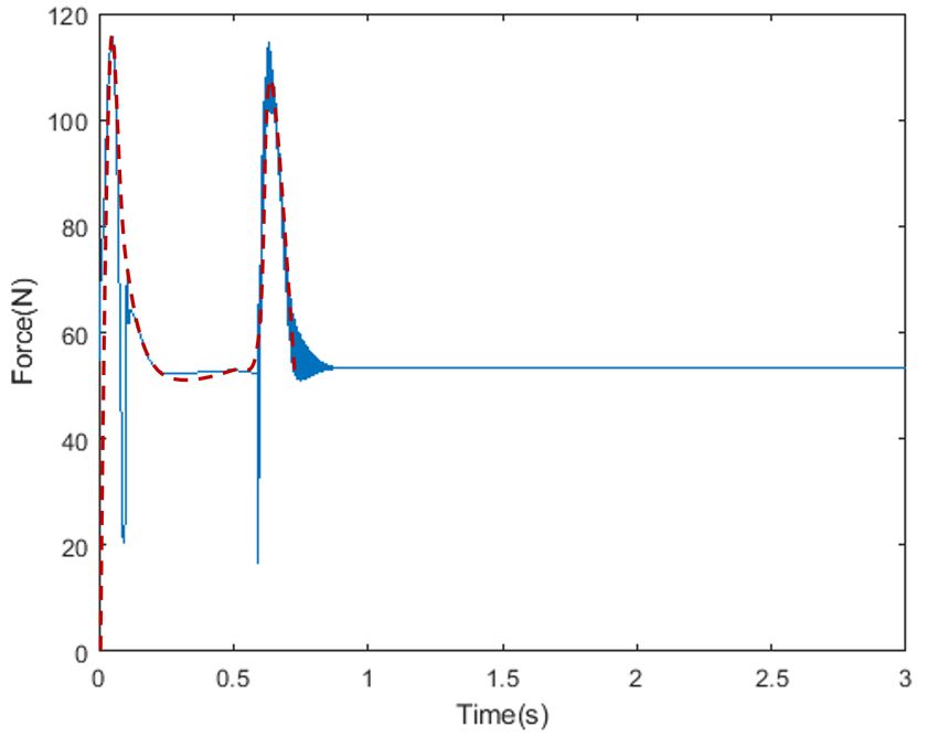
Sensors 2021, 21, 287                                                                                                            2 of 16

                                  without a Force/Torque (F/T) sensor. Moreover, the performance is modulated by inertia
                                  information. Park [22] proposed a hybrid approach for contact force control combining the
                                  null space method and observer. The approach removes the effect of disturbance or error
                                  with the F/T sensor [23] by applying a filter or observer to reduce noise from sensed signal.
                                  Furthermore, the observer can estimate the force for sensorless control [24]. However,
                                  these approaches have delays that significantly reduce the performance and stability of the
                                  robots. the F/T sensor for bipedal robots is also high cost and weighs over 500 g.

                         (a) ZMP controlled robot                                             (b) Human

      Figure 1. Swing leg’s foot trajectory of (a) robot and (b) human during gait cycle. Robot’s trajectory is from pre-developed
      robot [25]. Human gait is running at 3.56 m/s [26,27].

                                        Neural network (NN) learning is a useful method for unknown complicated mod-
                                  els [28,29]. NN-based hybrid position/force control was proposed by Passold [30] and
                                  Kumar [31]. Moreover, observer based approaches have been reported in [32–34]. How-
                                  ever, these researches also used a force sensor in their model. Unlike sensor based control,
                                  Xu [35] suggested an impedance control based on an observer without force sensor. Adap-
                                  tion algorithm is applied to estimate stiffness and position of environment. Yet, this model
                                  has a significant delay for early contact.
                                        In this paper, we propose a NN model to control ground reaction force without F/T
                                  sensor. This approach reduces modeling error and effort for finding model parameters.
                                  The contributions of our work are shown as follows:
                                  •     We propose a model based on neural network (NN) estimation on push-off force
                                        (GRF) control. It effectively decreases errors created by the robot’s mass and gravity.
                                  •     The neural network model is applied with Linear Quadratic Regulator (LQR), which is
                                        adopted for balancing and generating desired force for push-off.
                                  •     We introduce the simulation to prove that our approach is validated in dynamic
                                        situations like walking.
                                       The rest of the paper is organized as follows. Section 2 introduces the NN model and
                                  procedure of the simulation. Section 3 shows The results obtained from our model and
                                  simulation. The analysis about the result is summarized in Section 4. Section 5 concludes
                                  the paper.

                                  2. Method
                                  2.1. Neural Network Model
                                       The parallel type leg in this paper is shown in Figure 2. It is developed for reducing
                                  inertia and fast walking. Physical modeling and simulation are executed on the MATLAB
                                  Simscape. There are two motors on the hip to control the position (x,z) of the foot. The hip
                                  is connected to the body with a roll motor and is fixed during the NN training.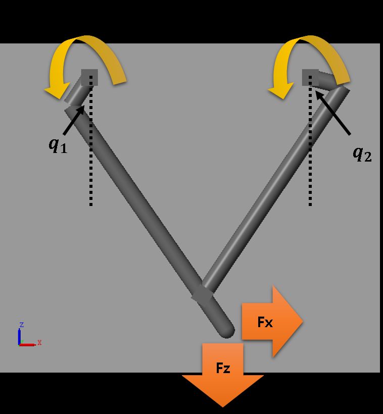
Sensors 2021, 21, 287                                                                                              3 of 16

                             Dynamic equation for leg can be formulated as:

                                                      I θ̈ + C (θ, θ̇ ) + Kθ + G (θ ) + J T F = τ                     (1)
                        where I is the inertia matrix, C represents the coriolis and centrifugal term, K is the stiffness
                        matrix and G (θ ) is the gravity function. The matrix J is the contact Jacobian for the contact
                        position and F is the contact force matrix. θ is the joint angle matrix and τ is the joint
                        torque matrix. If we the know exact model, the reference torque for the desired force is
                        obtained by:

                                          τre f erence = I θ̈m + C (θm , θ̇m ) + Kθm + G (θm ) + J T Fdesired         (2)
                        where θm represents the measured joint angle. Because the model information from CAD
                        is not perfect, we need to conduct experiments for calculating the exact parameter [18].
                        Besides, links must be decomposed, and the test takes much time and effort. Further-
                        more, if we use a force sensor or observer to compensate the modeling error, the delay
                        is unavoidable.

                        Figure 2. Leg model for neural network regression.

                            Thus, we propose a neural network model for removing model error without force
                        sensor. Because the inertia of the leg is negligible against the body in this model, I, C could
                        be omitted. Then, the reference torque is simplified by:

                                          τre f erence = Kθm + G (θm ) + J T Fdesired = h(q1 , q2 , Fdx , Fdz )       (3)
                        where q1 , q2 are the joint angle from the left and right motors, Fdx , Fdz represents the x-axis
                        and z-axis of the desired contact force. We assume the robot’s foot is fixed on a vertically
                        moving stage with a force sensor. When the torque (τ, τr ) is applied on the foot position by
                        the joint angle (q1 , q2 ), we could measure the generated force Fx , Fz .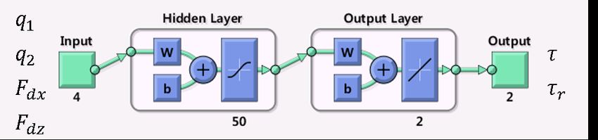
Sensors 2021, 21, 287                                                                                                 4 of 16

                                     Our purpose is to acquire an approximation function of h by using these data. The neu-
                               ral network is efficient for curve fitting and works well in nonlinear regression. To avoid
                               overfitting, the Bayesian regularization algorithm is adopted .
                                     In Figure 3 and 4, the torque surface is plotted to determine the neural network param-
                               eter. The figures show h is not a highly nonlinear function. Therefore, we used one hidden
                               layer. When the data are divided into 10 values in the range, sufficient performance is
                               achieved. 10,000 datasets are collected under each 10q1 × 10q2 × 10Fx × 10Fz . Performance
                               by random datasets is not significantly different. Ranges of input data are determined
                               as follows:
                                                                                  π                π
                                                     F ∈ [−100, 100] N, q1 ∈ [− , 0]rad, q2 ∈ [0, ]rad
                                                                                  2                2

                           (a) Left motor torque                                  (b) Right motor torque

                            Figure 3. Measured torque is plotted for each force, q1 = − 14
                                                                                        π
                                                                                           , q2 =    π
                                                                                                     14 .

                           (a) Left motor torque                                  (b) Right motor torque

                                                                                          100            100
                        Figure 4. Measured torque is plotted for each joint angle, Fx =    7 N, Fz   =    7 N.

                                     The structure of the NN model is described in Figure 5 and in Equation (4).

                                                                y = b2 + w L ∗ tansig(b1 + w I x )                       (4)
                                                               T
                               •      y = output vector = τ τr .
                               •      b1 , b2 = bias vector.
                               •      w L = Layer weight matrix, w I = Input weight matrix.
                               •      tansig(n) = 1+e2−2n − 1.
Sensors 2021, 21, 287 5 of 16
T
• x = input vector = q1 q2 Fdx Fdz .
Figure 5. Neural network model for regression.
We used 70% of the data for training, 5% for validation, and 25% for the test. The
parameters for NN learning are shown in Table 1. Training stops when the maximum
number of epochs is reached, µ exceeds µmax or the gradient falls below min_grad.
Table 1. Paratmeters used for neural network training.
Parameters Value Description
epochs 1000 Maximum number of epochs
µ 0.005 Marquardt adjustment parameter
µdec 0.1 Decrease factor for µ
µinc 10 Increase factor for µ
µmax 1 × 10¹⁰ Maximum value for µ
min_grad 1 × 10⁻⁷ Minimum performance gradient
Cad Model
The same approach is tested on a realistic CAD model. It contains a motor, gearbox
and it is fully designed for manufacturing. We assume this leg has the same workspace as
a pre-developed robot [25]. The leg length is twice as long. The motor is selected for an
increased length and weight. One motor position is changed because the motor is too big
to place side by side. The range of q1 is not symmetric because the length of the left and
right link are not the same.
Fx ∈ [−200, 200] N, Fz ∈ [−100, 1000] N, q1 ∈ [0.82q2 − 0.6067, 0.82q2 + 0.52]rad, q2 ∈ [0, 1.8]rad
2.2. Lqr Design
Figure 6 shows the 2D robot model and the parallel leg is simplified into a single
effective link. LQR is an optimal feedback controller for a linear plant, and is easily tuned
for multiple objectives by state (Q) and input (R) weight matrix.
The equations obtained from the model are shown below:
(
M ẍ = Fx cos(qb )
Mz̈ = Fz cos(qb ) − Mg for body
R x = − Fx cos(qb )
(5)
R
z = Mg − Fz cos(qb ) for leg
qb = ql − qh
I q¨ = R lcos(q ) − R lsin(q )
l x l z l
• M = mass of robot, g = gravity acceleration.
• F = force from leg to body.
• R = force from body to leg.
• qb = body angle, qh = hip angle, ql = leg angle.
• I = inertia of robot, l = length from body to foot.Sensors 2021, 21, 287 6 of 16
Figure 6. Free body diagram for body.
Besides high gain being applied in the support phase, we assume l is constant. The
1
mass of the leg is 20 scale of robot mass, thus it is ignored. At a linearized point, q?b = q?l ≈ 0.
The state-space equation for LQR can be written as:
H Ẋ = AX + BU
Ẋ = H −1 ( AX + BU ) = A0 X + B0 U
T
X = qb q˙b x ẋ z ż
H = diag( 1 I 1 M 1 M )
0 1 0 0 0 0
0 0 0 0 0 0
0 0 0 1 0 0
A= 0 0 0 0 0 0
(6)
0 0 0 0 0 1
0 0 0 0 0 0
0 0
− l 0
0 0
B= 1 0
0 0
0 1
T
U = Fx Fz
We use simple PD control on hip roll motors.
uroll = K P (qre f − qroll ) − K D q̇roll (7)
qroll = angle of roll motor, q̇roll = angular velocity of roll motor, qre f = reference angle
qre f is a constant that keeps initial hip roll angle.
100 10 50,000 5000 0 0
Klqr =
0 0 0 0 50,000 5000 (8)
U = −Klqr XSensors 2021, 21, 287 7 of 16
Klqr is calculated from (A, B, Q, R) by the algebric Riccati equation. The controllability
matrix is not full rank but is stabilizable. It means that the robot could fall from some
initial states. Controlling x and qb are trade-offs because two states are coupled. If we give
too much weight to x, qb is not controlled properly. After some simulation, we could find
appropriate ratio for them.
The entire control flow is described as:
1. LQR calculates desired contact force (Fx , Fz ) from error.
2. Desired Joint torque (τ, τr ) is obtained from a neural network regression model.
3. Apply the joint torque to the robot plant and measure the states.
Workflow is also described in Figure 7.
Figure 7. Entire control flow, NN means neural network model.
2.3. One Step Simulation
We establish a simulation model to verify that the proposed approach works well
while the robot body is moving. The robot model is demonstrated in Figure 8. There are
two hip roll motors on the invisible frame. The control objective for the hip roll motor is to
sustain the angle. There is no external constraint on the model, but only spatial contacts
between the spherical foot and ground. The static friction coefficient is 1 and the dynamic
is 0.8. This is the friction coefficient of rubber on dry concrete. The hip width is 0.1m and
the other parameters are written in Figure 9 and Table 2.
Figure 8. Robot model for simscape.Sensors 2021, 21, 287 8 of 16
Figure 9. Leg model parameter.
Table 2. Leg model parameter table.
Name Value
L1 (m) 0.04
L1r (m) 0.04
L2 (m) 0.24
L2r (m) 0.255
L f (m) 0.05
Lt (m) 0.08
M (kg) 10
Leg length parameters are optimized for minimizing the required torque, and the step
width is 0.1 m. The push-off force is generated by trajectory based on the trigonometric
function (pdesired = A2 (1 − cos( 2πt
T ))). The maximum force for the z-axis is 170% of the mass
and force for the x-axis is 40%. The step time and amplitude of the push-off is selected
by tuning.
Simulation starts from the double support phase. Right leg push-off ground and mode
is changed into a single support phase. Body angle and effective leg length l are regulated
in a single support phase. After heel-strike, the robot is balanced.
3. Results
3.1. Neural Network Model
We did the test to prove robustness:
1. Pick random desired force.
2. Calculate the joint torque by using a neural network model.
3. Compare the real torque for the desired force with a calculated one (Test 1).
4. Apply the joint torque and compare the measured force with the desired (Test 2).
Figure 10 shows the logarithmic MSE decrease as the number of neurons increases.
However, neurons more than 50 show negligible performance improvement in force
generation (Test 2). Thus, we decide the number of neurons is 50 and it needs about 27 ms
to calculate torque.Sensors 2021, 21, 287 9 of 16
(a) linear scale (b) log scale
Figure 10. Mean square error of torque by the number of neurons.
Test 1 executed 1000 times and Test 2 executed 100 times. When we use the Jacobian
method, torque is calculated by τre f erence = J T Fdesired . The gravitational term is not applied
because we assume the mass model is not accurate. In the error histogram (Figure 11a), the
torque error from the NN model is much lower than the error from the Jacobian method.
Table 3 shows the predicted torque error by dismissing I, C. In Test 2, the mean error from
the Jacobian method is 4.58 N and the mean error from NN is 0.37 N. The mean error is
reduced by 92% when a neural network model is applied.
(a) MSE of torque (red) Jacobian, (blue) NN (b) MSE of force prediction
Figure 11. Histogram of mean square error.
Table 3. Statistical value of prove test.
Test 1 (Nm) Test 2 (N)
MSE 9.45 × 10⁻⁵ 0.67
Mean 0.0039 0.37
STD 0.0089 0.74Sensors 2021, 21, 287 10 of 16
CAD Model
To prove the robustness of the NN model, Test 2 is applied to the CAD model. The root
mean squared error (RMSE) from the NN model is 73.7% lower than the Jacobian method.
Because the CAD model is heavier (4.5 kg) than simplified model (300 g), Figure 12 shows
increased force error. The moving average line indicates the error from NN is significantly
smaller than the Jacobian’s.
(a) Jacobian (b) Neural network
Figure 12. Force prediction error.
According to Figure 13 and Table 4, the average error is reduced by 85.6%. There
are some spikes over 10 N in the NN model. When the leg is almost fully stretched, the
spikes appear by a singularity. Simscape solver’s linearization and approximation also
make an error.
Figure 13. Histogram of force prediction error.Sensors 2021, 21, 287 11 of 16
Table 4. Statistical value of prove test in CAD model.
Error Max (N) Avg (N) Var (N) RMSE (N)
Jacobian 51 21.2 36.2 22.0
Neural 36 3.1 24.2 5.8
Change (%) −29.4 −85.6 −33.1 −73.7
3.2. One Step Simulation
Figure 14 demonstrates the procedure of one step simulation. Figure 15 indicates
the states and input of the LQR controller. Heel strike occurs at 0.6 s and the robot keeps
balance without additional stepping. On the other hand, Atrias has no ability to keep
balance at standstill [20]. It is critical for robots with manipulator.
Figure 14. Still shot of one step simulation.Sensors 2021, 21, 287 12 of 16
Figure 15a,b show the movement of the body, taking maximum overshoot values of
1 cm and 2 cm. Figure 15c shows the response of the body angle qb , which takes values
between −0.4 and 1.2 degrees. The joint torque of the swing foot, having maximum values
of −8 and 8 Nm, are presented in Figure 15d. Peak values appeared by mode transition
and numerical error of simulation.
(a) xbody (b) zbody
(c) qbody (d) Control input
Figure 15. States and input of swing foot.
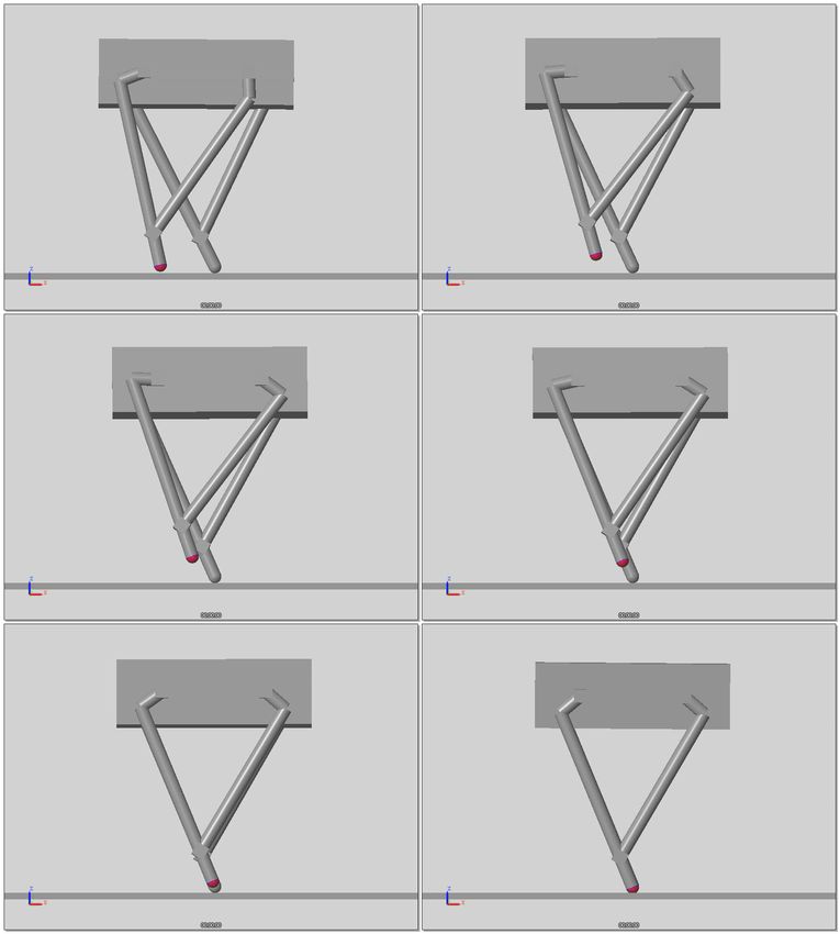
Figure 16 shows the real and target normal force of the stance leg. The NN model
operates normally under moving conditions. Average error is 0.64 N.
In Figure 17a, GRF is not measured in the swing phase. Human’s GRF is drawn for a
stance leg from heel strike to push-off [36]. It needs more steps to draw the grf of the stance
leg. Hence, we draw similar results by adding the swing and stance leg’s normal force.Sensors 2021, 21, 287 13 of 16
Figure 16. Measured and desired force.
(a) Swing leg’s forces (b) Normal force (Swing leg + stance leg)
Figure 17. Normal and friction force of one step simulation. Red dashed line: approximation of sum.
4. Discussion
The neural network model has a high accuracy in force control. The average and RMS
error are smaller than 10 N. According to Table 4, the proposed model achieves better
accuracy than the Jacobian method without including mass information. The NN model
removes the time-consuming process of formulating equations and finding the parameters
of each link. In biped robots, the error is produced by bolts, bearings, wire and electronic
parts. Even though all terms are modeled, force control error always exists [21]. NN
modeling is a systematic approach to modify models by experiments and learning. The
main reason for performance improvement comes from dismissing gravitational terms in
the Jacobian method. Since we designed the leg for faster movement, the leg mass under
5 Kg was used. There will be more improvement for heavier legs. In the manipulator’s case,
a computed torque method or observer based approach is applied for better performance
and removing the model error. Due to the noisy value from sensors, a filter or observer
is used in those approaches. Stability and performance deteriorate because the delay isSensors 2021, 21, 287 14 of 16
accompanied by filters. Unlike manipulators, walking robots could fall by a small delay.
F/T sensors for an observer are also expensive and heavy.
Since Equation (3) has no terms about ground, the NN model is not affected by the
condition and material of the ground. Therefore, the model is also working in a floating
state. Figure 3 shows the model is linear about Fz . Thus, Fz range for the dataset could
be from 0 to positive value. If we get data only for pushing ground, it does not have any
performance drop.
Based on the results in Section 3.2, our approach can be used for moving platforms.
Figure 17b shows an approximated line that resembles a human’s GRF. There is a flat part
between two peaks in the single support phase. Because the robot’s speed is 0.25 m/s
which is much slower than a human’s (1–1.5 m/s), using push-off, the robot could achieve
more speed for multiple step. Although push-off and heel strike are disturbances over
100 N, the proposed LQR controller rejects the disturbance with a small error. Robots could
stand without any motion or additional stepping. ZMP-controlled robots usually need an
F/T sensor or advanced control like a capture point to remove disturbance.
5. Conclusions
The purpose of this article is to provide a new contact force control algorithm. Un-
known disturbance and modeling error will cause the failure of the walking robot. We pro-
pose a NN based force control method to solve these problems. We use NN regression
to remove time-consuming steps like formulating equations and finding parameters for
model. Secondly, we introduce the LQR walking controller with the NN model for balanc-
ing and push-off.
The performance of contact force generation was compared with the Jacobian method.
The result shows that the neural network model significantly improves the performance
of force control. The research pointed out that the proposed method is highly applicable
for contact force control. Our approach has strong robustness on one step simulation
which contains transient disturbance. The proposed algorithm satisfies requirements under
simulation and the result shows the feasibility of applying our approach to walking control.
NN modeling can be easily implemented by other manipulators or robots. The ad-
vantage of these solutions can be exploited well on complicated multi-axis robots or
parallel manipulators.
In our future work, we will add frictional or damping terms in the model. Friction
modeling is a challenging problem to be added to force control. However, this is essential
to improve performance in walking of real robots. The redundant degree of freedom will
be considered later. Additional objects like torque minimization can be added to the model.
Author Contributions: Conceptualization, B.K. and S.K.; methodology, B.K.; software, B.K.; writing—
original draft preparation, B.K.; writing—review and editing, B.K. All authors have read and agreed
to the published version of the manuscript.
Funding: This research was funded by Korea Hydro & Nuclear Power Co., Ltd. Project name is
‘Development of Visual Inspection Robot for Essential Service Water Piping’ grant number N06200049.
Institutional Review Board Statement: Not applicable.
Informed Consent Statement: Not applicable.
Data Availability Statement: Data available on request due to restrictions by funding organization.
Conflicts of Interest: The authors declare no conflict of interest.Sensors 2021, 21, 287 15 of 16
Abbreviations
The following abbreviations are used in this manuscript:
NN Neural Network
GRF Ground Reaction Force
CoM Center of Mass
LQR Linear Quadratic Regulator
F/T Force Torque
CAD Computer Aided Design
ZMP Zero Moment Point
References
1. Morisawa, M.; Kajita, S.; Kanehiro, F.; Kaneko, K.; Miura, K.; Yokoi, K. Balance control based on Capture Point error compensation
for biped walking on uneven terrain. In Proceedings of the 2012 12th IEEE-RAS International Conference on Humanoid Robots
(Humanoids 2012), Osaka, Japan, 29 November–1 December 2012; pp. 734–740. [CrossRef]
2. Englsberger, J.; Ott, C. Integration of vertical COM motion and angular momentum in an extended Capture Point tracking
controller for bipedal walking. In Proceedings of the 2012 12th IEEE-RAS International Conference on Humanoid Robots
(Humanoids 2012), Osaka, Japan, 29 November–1 December 2012; pp. 183–189. [CrossRef]
3. Shafiee-Ashtiani, M.; Yousefi-Koma, A.; Shariat-Panahi, M.; Khadiv, M. Push recovery of a humanoid robot based on model
predictive control and capture point. In Proceedings of the 2016 4th International Conference on Robotics and Mechatronics
(ICROM), Tehran, Iran, 26–28 October 2016; pp. 433–438. [CrossRef]
4. Sugihara, T.; Yamamoto, T. Foot-guided agile control of a biped robot through ZMP manipulation. In Proceedings of the 2017
IEEE/RSJ International Conference on Intelligent Robots and Systems (IROS), Vancouver, BC, Canada, 24–28 September 2017;
pp. 4546–4551. [CrossRef]
5. Ishiguro, Y.; Kojima, K.; Sugai, F.; Nozawa, S.; Kakiuchi, Y.; Okada, K.; Inaba, M. Bipedal oriented whole body master-slave system
for dynamic secured locomotion with LIP safety constraints. In Proceedings of the 2017 IEEE/RSJ International Conference on
Intelligent Robots and Systems (IROS), Vancouver, BC, Canada, 24–28 September 2017; pp. 376–382. [CrossRef]
6. Kuindersma, S.; Permenter, F.; Tedrake, R. An efficiently solvable quadratic program for stabilizing dynamic locomotion.
In Proceedings of the 2014 IEEE International Conference on Robotics and Automation (ICRA), Hong Kong, China, 31 May–7 June
2014; pp. 2589–2594. [CrossRef]
7. Caron, S.; Pham, Q.; Nakamura, Y. ZMP Support Areas for Multicontact Mobility Under Frictional Constraints. IEEE Trans. Robot.
2017, 33, 67–80. [CrossRef]
8. Kamioka, T.; Kaneko, H.; Takenaka, T.; Yoshiike, T. Simultaneous Optimization of ZMP and Footsteps Based on the Analytical
Solution of Divergent Component of Motion. In Proceedings of the 2018 IEEE International Conference on Robotics and
Automation (ICRA), Brisbane, Australia, 21–25 May 2018; pp. 1763–1770. [CrossRef]
9. Kim, J.H.; Lee, J.; Oh, Y. A Theoretical Framework for Stability Regions for Standing Balance of Humanoids Based on Their LIPM
Treatment. IEEE Trans. Syst. Man Cybern. Syst. 2020, 50, 4569–4586. [CrossRef]
10. Yu, Z.; Zhou, Q.; Chen, X.; Li, Q.; Meng, L.; Zhang, W.; Huang, Q. Disturbance Rejection for Biped Walking Using Zero-Moment
Point Variation Based on Body Acceleration. IEEE Trans. Ind. Inform. 2019, 15, 2265–2276. [CrossRef]
11. Kajita, S.; Kanehiro, F.; Kaneko, K.; Fujiwara, K.; Harada, K.; Yokoi, K.; Hirukawa, H. Biped walking pattern generation by using
preview control of zero-moment point. In Proceedings of the IEEE International Conference on Robotics and Automation, Taipei,
Taiwan, 14–19 September 2003; Volume 2, pp. 1620–1626. [CrossRef]
12. Zelik, K.E.; Takahashi, K.Z.; Sawicki, G.S. Six degree-of-freedom analysis of hip, knee, ankle and foot provides updated
understanding of biomechanical work during human walking. J. Exp. Biol. 2015, 218, 876–886. [CrossRef] [PubMed]
13. Soo, C.H.; Donelan, J.M. Mechanics and energetics of step-to-step transitions isolated from human walking. J. Exp. Biol. 2010,
213, 4265–4271. [CrossRef]
14. Collins, S. Dynamic Walking Principles Applied to Human Gait. Ph.D. Thesis, The University of Michigan, Ann Arbor, MI,
USA, 2008.
15. Huang, T.W.; Shorter, K.; Adamczyk, P.; Kuo, A. Mechanical and energetic consequences of reduced ankle plantarflexion in
human walking. J. Exp. Biol. 2015, 218. [CrossRef]
16. Collins, S.; Kuo, A. Recycling Energy to Restore Impaired Ankle Function during Human Walking. PLoS ONE 2010, 5, e9307.
[CrossRef]
17. Zelik, K.E. Is the Foot Working With or Against the Ankle During Human Walking? In Proceedings of the Dynamic Walking
Conference, Columbus, OH, USA, 21–24 July 2015.
18. Park, H.W.; Sreenath, K.; Hurst, J.; Grizzle, J. Identification of a Bipedal Robot with a Compliant Drivetrain. IEEE Control Syst.
2011, 31, 63–88. [CrossRef]
19. Spring-Mass Walking with ATRIAS in 3D: Robust Gait Control Spanning Zero to 4.3 KPH on a Heavily Underactuated Bipedal
Robot. In Proceedings of the ASME 2015 Dynamic Systems and Control Conference, Columbus, OH, USA, 28–30 October 2015.Sensors 2021, 21, 287 16 of 16
20. Hubicki, C.M.; Abate, A.; Clary, P.; Rezazadeh, S.; Jones, M.S.; Peekema, A.; Why, J.V.; Domres, R.; Wu, A.; Martin, W.; et al.
Walking and Running with Passive Compliance: Lessons from Engineering: A Live Demonstration of the ATRIAS Biped.
IEEE Robot. Autom. Mag. 2018, 25, 23–39. [CrossRef]
21. Lee, Y.; Hwang, S.; Park, J. Balancing of humanoid robot using contact force/moment control by task-oriented whole body
control framework. Auton. Robots 2016, 40. [CrossRef]
22. Park, J.; Khatib, O. Robot multiple contact control. Robotica 2008, 26, 667–677. [CrossRef]
23. Bouyarmane, K.; Chappellet, K.; Vaillant, J.; Kheddar, A. Quadratic Programming for Multirobot and Task-Space Force Control.
IEEE Trans. Robot. 2019, 35, 64–77. [CrossRef]
24. Nagai, S.; Kawamura, A. Position/Force Sensorless Force Control Using Reaction Force Observer for Compact Dual Solenoid
Actuator. In Proceedings of the IECON 2019—45th Annual Conference of the IEEE Industrial Electronics Society, Lisbon, Portugal,
14–17 October 2019; Volume 1, pp. 3635–3640. [CrossRef]
25. Song, B. The Robot For Nuclear Plant. Korea JoongAng Daily, 26 April 2018. Available online: https://news.joins.com/article/22
569622 (accessed on 31 December 2020).
26. Dorn, T.; Lin, Y.C.; Pandy, M. Estimates of muscle function in human gait depend on how foot-ground contact is modelled.
Comput. Methods Biomech. Biomed. Eng. 2011, 15, 657–668. [CrossRef] [PubMed]
27. Dorn, T.; Schache, A.; Pandy, M. Muscular strategy shift in human running: Dependence of running speed on hip and ankle
muscle performance. J. Exp. Biol. 2012, 215, 1944–1956. [CrossRef]
28. Lewis, F.; Ge, S. Neural Networks in Feedback Control Systems; John Wiley & Sons, Inc.: Hoboken, NJ, USA, 2006; pp. 791–825.
[CrossRef]
29. Puga-Guzmán, S.; Moreno-Valenzuela, J.; Santibañez, V. Adaptive Neural Network Motion Control of Manipulators with
Experimental Evaluations. Sci. World J. 2014, 2014, 694706. [CrossRef] [PubMed]
30. Passold, F.; Stemmer, M. Force Control of a Scara Robot Using Neural Networks. In Proceedings of the Fourth International
Workshop on Robot Motion and Control (IEEE Cat. No.04EX891), Puszczykowo, Poland, 20 June 2004; pp. 247–252. [CrossRef]
31. Kumar, N.; Panwar, V.; Nagarajan, S.; Sharma, S.; Borm, J.H. Neural network based hybrid force/position control for robot
manipulators. Int. J. Precis. Eng. Manuf. 2011, 12, 419–426. [CrossRef]
32. Piao, J.; Kim, E.S.; Choi, C.S.; Moon, C.B.; Park, M.H. Indirect Force Control of a Cable-Driven Parallel Robot: Tension Estimation
using Artificial Neural Network trained by Force Sensor Measurements. Sensors 2019, 19, 2520. [CrossRef]
33. Wahrburg, A.; Bös, J.; Listmann, K.D.; Dai, F.; Matthias, B.; Ding, H. Motor-Current-Based Estimation of Cartesian Contact Forces
and Torques for Robotic Manipulators and Its Application to Force Control. IEEE Trans. Autom. Sci. Eng. 2018, 15, 879–886.
[CrossRef]
34. Li, C.; Zhang, Z.; Xia, G.; Xie, X.; Zhu, Q. Efficient Force Control Learning System for Industrial Robots Based on Variable
Impedance Control. Sensors 2018, 18, 2539. [CrossRef]
35. Xu, W.; Cai, C.; Zou, Y. Neural-network-based robot time-varying force control with uncertain manipulator–environment system.
Trans. Inst. Meas. Control 2014, 36, 999–1009. [CrossRef]
36. Geyer, H.; Seyfarth, A.; Blickhan, R. Compliant leg behavior explains basic dynamics of walking and running. Proc. Biol. Sci.
R. Soc. 2006, 273, 2861–2867. [CrossRef] [PubMed]You can also read