Investigation by Digital Image Correlation of Mixed Mode I and II Fracture Behavior of Metallic IASCB Specimens with Additive Manufactured ...
←
→
Page content transcription
If your browser does not render page correctly, please read the page content below
metals
Article
Investigation by Digital Image Correlation of Mixed
Mode I and II Fracture Behavior of Metallic IASCB
Specimens with Additive Manufactured
Crack-Like Notch
Ivo Campione 1 , Tommaso Maria Brugo 2 , Giangiacomo Minak 1 , Jelena Janković Tomić 3 ,
Nebojša Bogojević 3 and Snežana Ćirić Kostić 3, *
 1   Department of Industrial Engineering (DIN), Via Fontanelle 40, 47121 Forlì, Italy;
     ivo.campione@unibo.it (I.C.); giangiacomo.minak@unibo.it (G.M.)
 2   Department of Industrial Engineering (DIN), University of Bologna, 40136 Bologna, Italy;
     tommasomaria.brugo@unibo.it
 3   Faculty of Mechanical and Civil Engineering in Kraljevo, University of Kragujevac, 36000 Kraljevo, Serbia;
     tomic.j@mfkv.rs (J.J.T.); bogojevic.n@mfkv.rs (N.B.)
 *   Correspondence: cirickostic.s@mfkv.kg.ac.rs; Tel.: +381-0648938826

 Received: 11 February 2020; Accepted: 17 March 2020; Published: 20 March 2020

 Abstract: This work investigates the fracture behavior of maraging steel specimens manufactured
 by the selective laser sintering (SLS) technology, in which a crack-like notch (sharp notch) was
 directly produced during the additive manufacturing (AM) process. For the evaluation of the fracture
 toughness, the inclined asymmetrical semi-circular specimen subjected to three points loading (IASCB)
 was used, allowing to cover a wide variety of Mode I and II combinations. The effectiveness of
 manufacturing crack-like notches via the SLS technique in metals was evaluated by comparing the
 obtained experimental results with the ones obtained with pre-cracks induced by fatigue loading.
 The investigation was carried out by using the digital image correlation (DIC) technique, that allowed
 the evaluation of the full displacement fields around the crack tip. The displacement field was then
 used to compute the stress intensity factors (SIFs) for various combinations of Mode I and II, via a
 fitting technique which relies on the Williams’ model for the displacement. The SIFs obtained in this
 way were compared to the results obtained with the conventional critical load method. The results
 showed that the discrepancy between the two methods reduces by ranging from Mode I to Mode II
 loading condition. Finally, the experimental SIFs obtained by the two methods were described by the
 mixed mode local stress criterium.

 Keywords: additive manufacturing; selective laser sintering; maraging steel; fracture toughness;
 stress intensity factors; mixed mode I-II; IASCB specimens; digital image correlation; Williams’ model;
 local stress criterium

1. Introduction
     Additive manufacturing (AM) is a powerful technique that allows one to manufacture complex
geometries, which would be difficult or impossible to obtain with the traditional subtractive techniques.
Among the AM techniques, selective laser sintering (SLS) is one of the most widespread. It exploits
a laser beam to sinter powder to build objects bottom-up, layer-by-layer and has the advantage
of being applicable to a large variety of materials [1] such as metals, polymers, ceramics or wax.
However, one drawback of the SLS technique is that the mechanical properties of the product depend
on the direction in which the geometry is built up, which is to be properly chosen, especially when

Metals 2020, 10, 400; doi:10.3390/met10030400                                      www.mdpi.com/journal/metals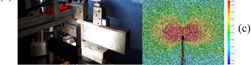
Metals 2020, 10, 400                                                                               2 of 13

designing structural components [2]. This work investigates the fracture mechanics properties of
SLS metallic materials and the capability of the AM processes to build 3-D artificial crack-like notch
into them. This less conventional method could be used to induce internal crack-like notches in
the specimens and study three-dimensional fracture mechanics problems, which are difficult to be
tackled by conventional methods. Previous study of T. Brugo et al. [3] on fracture toughness of
AM Polyamide materials have shown that it is possible to intentionally induce crack-like notches in
any desired direction during the AM process and that the building direction slightly influences the
fracture toughness.
     In literature, several configurations are proposed to investigate mixed mode I/II fracture behavior.
Two main types of configurations can be found: the first one exploits the use of asymmetrical
rectangular specimens, such as [4,5] or the modified compact tension (CT) specimen [6]. The second
one involves the use of disc-like specimens, such as the Brazilian Disc (BD) [7], the Semi-Circular Bend
(SCB) [8] specimen, the Asymmetric Semi-Circular Bend (ASCB) [9,10] specimen and the Inclined edge
cracked Semi-Circular Bend (IASCB) [11,12] specimen. In this work the IASCB specimen, subjected to
three-point bend loading, was utilized (the test configuration is described in detail in § 2.2). This
specimen, compared to the other ones reported, gives the opportunity to cover a wider range of the
stress intensity factors (KI and KII ) and T-Stress without requiring a complicated loading fixture.
     IASCB specimens were manufactured by SLS with different crack-like notch angles and compared
with others in which the crack was induced by fatigue loading, considering different values of
support spans. To evaluate the fracture behavior, the digital image correlation technique (DIC) was
exploited. Along with the electronic speckle pattern interferometry (ESPI) [13], the DIC is one of the
most widespread optical technique that allows to easily and cheaply measure the full displacement
and strain field [14]. It requires just a camera of sufficiently high resolution and an algorithm to
perform the correlation between the images, which is carried out by exploiting a speckle pattern
(usually spray-painted) on the surface of the sample. This pattern serves as an aid for the correlation
algorithm, which relies on matching subsets of pixels in consecutive images: the location of a point in
an undeformed subset is found in the deformed image, and the displacement can thus be determined.
     By means of this technique, the displacement field is computed directly, whereas the strain
field is calculated by numerical differentiation of the former, with inevitable introduction of noise.
Mainly for this reason, fitting methods usually exploit the displacement field rather than the strain
one. In fracture mechanics, these displacement fields, other than providing a complete qualitative
insight on the material behavior in the zone of interest (namely the crack tip, in the case study) can
be used to quantitatively characterize the fracture behavior of the material. In particular, they can be
exploited to estimate the stress intensity factors (SIFs). One notable work in this direction was done
by McNeill et al. [15] who tested CT and Three Point Bending (3PB) specimens, and compared the
results between DIC and analytical data, suggesting a methodology to use the DIC data to determine
the fracture toughness KIC of specimens. In general, two main approaches emerges in literature
concerning the fitting of theoretical models on the full displacement fields: the first one is based on
guessing a general form of an analytical function and fitting this to the displacement experimental data:
an example is the complex function analysis of Muskhelishvili [16], which was further developed to
calculate mixed mode (I + II) [17] and generalized to cases without restrictions in boundary conditions
or symmetry [18]. The second approach is based on the Williams’ model [19–22], where the fitting
on the experimental data is done by considering the first n term of the Williams expansion for the
displacement. In this work this latter approach was used. The SIFs obtained by the DIC fitting were
compared to the ones obtained with the conventional critical load method. Finally, the resulting SIFs
were described by the mixed mode local stress criterium.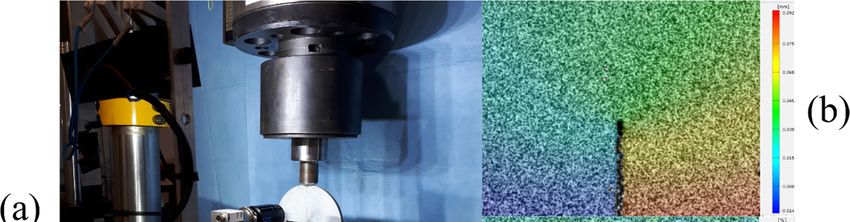
Metals 2020, 10, 400 3 of 13
Metals 2020, 10, x FOR PEER REVIEW 3 of 14
2. Materials andThe specimens were manufactured by the EOSINT M 280 SLS machine (EOS GmbH Electro
Methods
Optical Systems, Krailling/Munich, Germany), using the EOS Maraging Steel MS1 steel powder, with
a chemical composition corresponding to the European 1.2709 classification. The process parameters
2.1. Specimenwere
Fabrication by Additive
set as described Manufacturing
in [23] and as advised by the SLS machine manufacturer.
In particular, the layer thickness was set to 40 μm and the scanning pattern of each layer was
The specimens werethemanufactured
rotated around vertical axis withby the EOSINT
respect M 280
to the previous one, SLS machine
in order to reduce(EOS GmbH Electro
in-plane
Optical Systems, Krailling/Munich,
anisotropy. Germany),
After the laser sintering process,using the EOS
the specimens Maraging
underwent Steel
a surface MS1 treatment
cleaning steel powder, with a
by micro shot-peening,
chemical composition followed to
corresponding by the
an ageing treatment
European by a heating
1.2709 in air up to The
classification. 490 °Cprocess
for 6 h, parameters
followed again by micro shot-peening. According to the powder supplier, after the age-hardening
were set as described in [23]
treatment, the andanisotropy
material as advised can by
be the SLS machine
completely removed, manufacturer.
and the excellent mechanical
In particular, thedescribed
properties layer thickness
in Table 1 canwas set to 40 µm and the scanning pattern of each layer was
be attained.
rotated around the vertical axis with respect to the previous one, in order to reduce in-plane anisotropy.
Table 1. Mechanical properties of the specimens.
After the laser sintering process, the specimens underwent a surface cleaning treatment by micro
Property Value
shot-peening, followed by an ageing Sintered
treatmentDensityby a heating air up to 490 ◦ C for 6 h, followed
in g/cm³
8.0–8.1
again by micro shot-peening. According Elastic
toModulus
the powder supplier, 180 ± 20 after
GPa the age-hardening treatment,
Yield Strength min. 1862 MPa
the material anisotropy can be completely removed,
Tensile Strength and the excellent
min. 1930 MPamechanical properties described
in Table 1 can be attained. Hardness typ. 50–56 HRC
Ductility (Notched Charpy Impact Test) 11 ± 4 J
2.2. IASB Specimens
Table 1. Mechanical properties of the specimens.
The IASCB specimen, shown in Figure 1 is a semi-circular disk of radius
Property ValueR and thickness t which
contains a radial edge crack of length a, tilted with respect to the load direction of an angle α [11]. The
specimens were manufactured Sintered
by the Density
SLS technique with the built plane8.0–8.1 g/cmto3 the plane of the
parallel
Elastic Modulus
semi-circumference of the specimen. 180 ± 20 GPa
To conduct the fracture Yield Strength
tests, the specimens were located on two min.bottom
1862 supports
MPa and loaded
by a vertical force P. The existence
TensileofStrength
different geometric parameters allows
min. various
1930 MPacombinations of
Mode I and Mode II to be easilyHardness
achieved. The geometrical parameters typ.which
50–56canHRCbe varied to achieve
mixed mode (I and II) are:
Ductility (Notched Charpy Impact Test) 11 ± 4 J
1) S1/R and S2/R (the ratio between the support spans and the specimen radius);
2) a/R (the ratio between the crack length and the specimen radius);
2.2. IASB Specimens3) α (the angle between the crack line and the load direction).
In order to obtain the various mode combinations, only the parameters S2/R and α were varied.
S1 was
The IASCB maintained fixed
specimen, shownat 42in
mm, whereas
Figure 1 the
is avalues of t, R and a were
semi-circular disktheofsame for allR
radius theand
specimens
thickness t which
(t = 6mm, R= 60 mm, a = 24 mm) The various combinations of these two, indeed, can cover Mode I,
contains a radial edge crack of length a, tilted with respect to the load direction of an angle α [11].
Mode II and mixed modes I-II. When the bottom supports are located symmetrically to the crack line
The specimens(i.e.,were
when Smanufactured
1 = S2) and the crackby
linethe
is in SLS technique
the same direction aswith the(i.e.,
the load built
whenplane
α = 0°),parallel to the plane of
the specimen
is subjected to Mode
the semi-circumference of the specimen.I (opening mode). To obtain mixed mode I-II or Mode II (sliding mode), an
appropriate combination of S2/R and α should be chosen.
Figure 1. Geometrical parameters and loading conditions of the IASCB (Inclined edge cracked Semi-
Figure 1. Geometrical parameters and loading conditions of the IASCB (Inclined edge cracked
Circular Bend) specimen.
Semi-Circular Bend) specimen.
To conduct the fracture tests, the specimens were located on two bottom supports and loaded
by a vertical force P. The existence of different geometric parameters allows various combinations of
Mode I and Mode II to be easily achieved. The geometrical parameters which can be varied to achieve
mixed mode (I and II) are:
(1) S1 /R and S2 /R (the ratio between the support spans and the specimen radius);
(2) a/R (the ratio between the crack length and the specimen radius);
(3) α (the angle between the crack line and the load direction).
In order to obtain the various mode combinations, only the parameters S2 /R and α were varied.
S1 was maintained fixed at 42 mm, whereas the values of t, R and a were the same for all the specimens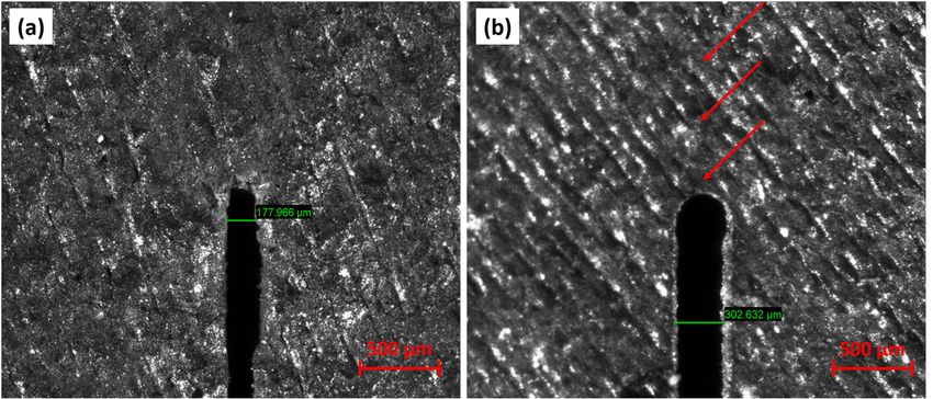
Metals 2020, 10, 400 4 of 13
(t = 6mm, R= 60 mm, a = 24 mm) The various combinations of these two, indeed, can cover Mode
I, Mode II and mixed modes I-II. When the bottom supports are located symmetrically to the crack
line (i.e., when S1 = S2 ) and the crack line is in the same direction as the load (i.e., when α = 0◦ ),
the specimen is subjected to Mode I (opening mode). To obtain mixed mode I-II or Mode II (sliding
mode), an appropriate combination of S2 /R and α should be chosen.
The notch was initiated in two different ways: 16 samples had the crack-like notch manufactured
during the additive manufacturing process (henceforth named AM specimens), while the remaining
3 samples had the
Metals notch
2020, 10, x FORinitiated
PEER REVIEW afterwards, by subtractive manufacturing (henceforth 4 of 14 named SM
specimens). In the SM specimens, the notch was induced by wire electrical discharge machining (EDM)
The notch was initiated in two different ways: 16 samples had the crack-like notch manufactured
technique; they
during were then fatigue
the additive pre-cracked
manufacturing (loading
process (henceforth ratio
named = KImin /K
AMrspecimens), Imax
while the=remaining
0.3) until the crack
propagated for 2 mm. In Figure 2 micrographs of the notch induced with the two different
3 samples had the notch initiated afterwards, by subtractive manufacturing (henceforth named SM methods
specimens). In the SM specimens, the notch was induced by wire electrical discharge machining
are shown. The crack-like notch induced by the AM technique has a radius of about 90 µm, whereas
(EDM) technique; they were then fatigue pre-cracked (loading ratio r = KImin/KImax = 0.3) until the crack
the notch induced
propagatedby SM for 2 has
mm. aInradius
Figure 2 of about 150
micrographs µm.
of the The
notch AM with
induced specimens were manufactured
the two different methods with
an angle α of 0 and 10 and tested with different support spans S1 and S2 (see Figure 1), in order
are ◦
shown. The ◦ crack-like notch induced by the AM technique has a radius of about 90 μm, whereas
the notch induced by SM has a radius of about 150 μm. The AM specimens were manufactured with
to obtain different mode combinations. The AM specimens with crack-like notch angle α of 0◦ were
an angle α of 0° and 10° and tested with different support spans S1 and S2 (see Figure 1), in order to
only tested with
obtain symmetric
different mode support spans
combinations. Theto
AMpre-crack
specimens and then monotonic
with crack-like notch angle αloaded inonly
of 0° were Mode I. Table 2
tested with tested
reports the specimens symmetric support
with spans to pre-crack
the method employed and then monotonic
to induce loadedthe
cracks, in Mode
values I. Table
of α,2 the supports
reports the specimens tested with the method employed to induce cracks, the values of α, the supports
spans and thespans
mixed mode ratio expressed as Me =
and the mixed mode ratio expressed as
2/πatan(K /K ).
= 2⁄ atan( ⁄ I). II
Figure 2. Micrographs of the crack tip; (a) crack-like notch manufactured during the additive
Figure 2. Micrographs of the crack tip; (a) crack-like notch manufactured during the additive
manufacturing process (AM) and (b) crack induced by subtractive manufacturing (SM) and
manufacturing processpre-cracking
subsequent (AM) and(indicated
(b) crack induced
by red arrows).by subtractive manufacturing (SM) and subsequent
pre-cracking (indicated by red arrows).
Table 2. Values of the geometrical parameters of the specimens tested.
Table 2. Values
Typeof the geometrical
α (deg) S2 (mm) Sparameters
1 (mm) n of the specimens
Mode Me tested.
SM 0 42 42 3 Mode I 1
Type α (deg)
AM S20 (mm) 42 S1 (mm)
42 3 n Mode I Mode
1 Me
AM 10 42 42 3 Mixed I-II 0.77
SM 0 AM 10 42 42 4218 3 3Mixed I-IIMode
I 0.48 1
AM 0 AM 10 42 42 42
10.2 3 3Mode II Mode
I 0.12 1
AM 10 42 42 3 Mixed I-II 0.77
2.3. Experimental
AM Setup10 42 18 3 Mixed I-II 0.48
TheAM
fracture tests10were performed
42 in displacement
10.2 control
3 at a speed
Modeof 1IImm/min,
0.12
by using a
hydraulic tensile machine Instron 8033 (Instron, Norwood, MA, USA) equipped with a 250 kN load
cell. The setup was arranged as shown in Figure 3. The 2D DIC system, used to measure the full
2.3. Experimental Setup field around the crack tip (in a window of 14 mm × 10 mm), consisted in a 10 MP Basler
displacement
ace acA3800-14uc camera (Basler, Ahrensburg, Germany) equipped with Basler lens C125-2522-5M-
The fracture tests were performed in displacement control at a speed of 1 mm/min, by using a
P f25mm (Basler, Ahrensburg, Germany) and two custom 40W 6000 K led lamps. The images were
hydraulic tensile machine
acquired at 2 Hz withInstron 8033Snap
the GOM (Instron,
2D free Norwood, MA, USA)
software and processed equipped
by GOM with
Correlate (GOM a 250 kN load
GmbH, Braunschweig, Germany, https://www.gom.com/), with the correlation
cell. The setup was arranged as shown in Figure 3. The 2D DIC system, used to measure the full parameters set as
follows: facet size of 19 pixel, point distance of 16 pixel, and spatial and temporary filter (median) set
displacementtofield
8 andaround the crack
3 respectively. tip (in a parameters
The correlation window of were mm ×based
14chosen 10 mm),
on the consisted
experimentalinDIC a 10 MP Basler
ace acA3800-14uc camera
optimization work(Basler, Ahrensburg,
of Palanca et al. [24] as Germany) equipped
the best compromise withprecision
between Basler andlensspatial
C125-2522-5M-P
f25mm (Basler,resolution, to evaluateGermany)
Ahrensburg, the displacement
andfield
twonear the crack40W
custom tip. In 6000
order to
Kmake the digital The
led lamps. imageimages were
correlation possible, a black speckle pattern with a white background was spray-painted on the
acquired at 2 specimens.
Hz with Figure
the GOM Snap
3b,c show 2D freeofsoftware
an example and
the correlated processed
displacement bystrain
and GOM fieldCorrelate
normal to the (GOM GmbH,
Braunschweig, crackGermany, https://www.gom.com/),
axis, correlated by the DIC software. with the correlation parameters set as follows:
facet size of 19 pixel, point distance of 16 pixel, and spatial and temporary filter (median) set to 8 and 3
respectively. The correlation parameters were chosen based on the experimental DIC optimization
work of Palanca et al. [24] as the best compromise between precision and spatial resolution, to evaluate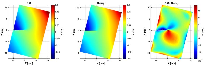
Metals 2020, 10, 400                                                                                                                   5 of 13

the displacement field near the crack tip. In order to make the digital image correlation possible, a
black speckle pattern with a white background was spray-painted on the specimens. Figure 3b,c show
an example of the correlated displacement and strain field normal to the crack axis, correlated by the
DIC software.Metals 2020, 10, x FOR PEER REVIEW                                      5 of 14

      Figure 3. (a) Experimental        setup;setup;
                    Figure 3. (a) Experimental  (b) crack    axis
                                                      (b) crack axisnormal   displacement
                                                                     normal displacement and (c)and
                                                                                                 strain(c) strain
                                                                                                        field       fieldbycorrelated by
                                                                                                              correlated
      the GOM software
                    the GOM around
                               software the crack
                                        around      tip, tip,
                                               the crack  forfor
                                                              Mode
                                                                 ModeI. I.

3. Results       3. Results

                 3.1. Evaluation of Stress Intensity Factors by the Critical Fracture Load Method
3.1. Evaluation of Stress Intensity Factors by the Critical Fracture Load Method
                       For the IASCB specimens, the stress intensity factor in mixed modes I-II were determined by
             exploitingspecimens,
     For the IASCB     the finite element
                                       themethod presented
                                            stress          [10]. According
                                                    intensity     factor into mixed
                                                                              this method, the loading
                                                                                       modes           conditions
                                                                                                  I-II were   determined by
             can be written as shown in Equations (1) and (2).
exploiting the finite element method presented [10]. According to this method, the loading conditions
can be written as shown in Equations (1)       = and (2).( ⁄ , 1⁄ , 2⁄ , )                                  (1)
                                                  2

                                                  =              ( ⁄ , 1⁄ , 2⁄ , )                                     (2)
                                                      2P
                                                           p
                                            KI =               πaYI (a/R, S1/R, S2/R, α)                                                   (1)
               where YI and YII are geometry factors2Rt corresponding to Mode I and Mode II, respectively (reported
               in Table 2 of reference [10]). Concerning the crack length a, for the SM specimens it was measured
                                                     P p  to πaY
                                                                  II (a/R, S1/R, S2/R, α)
               from the bottom of the K    sharp   notch     the pre-crack   tip, whereas for the AM specimens it was
                                            II =                                                                                  (2)
                                                    2Rt notch. For each test, the critical fracture load (Pcr) from the
               considered as the length of the crack-like
where YI andload-displacement
                YII are geometry   curves was evaluated at the instant in which the crack propagation was visually
                                         factors corresponding to Mode I and Mode II, respectively (reported in
               observed,  by the camera pointing at the crack tip. Then, by Equations (1) and (2) the critical stress
Table 2 of reference
               intensity[10]).
                         factorsConcerning         thetested
                                 (KI and KII) of the    crackIASCB
                                                                length    a, for the
                                                                       specimens  wereSM  specimens
                                                                                       calculated.      it was fracture
                                                                                                   The obtained  measured from the
bottom of theparameters    from the
                 sharp notch          critical
                                  to the       fracture load
                                            pre-crack         method
                                                           tip, whereas(henceforth named
                                                                             for the  AMPCR)    are reported
                                                                                            specimens        in Table
                                                                                                          it was      3.
                                                                                                                   considered as the
length of the 3.2.
                crack-like   notch. For each test, the critical fracture load (Pcr ) from the load-displacement
                   Evaluation of Stress Intensity Factors by the DIC Full Displacement Field
curves was evaluated        at   the instant in which the crack propagation was visually observed, by the
                    To model the displacement near the crack tip, the Williams’ asymptotic formulation [25] was
camera pointing      at the
               exploited. Thecrack
                                u and tip.
                                         v areThen,     by Equations
                                                the displacement            (1) crack
                                                                     along the   and (2)
                                                                                       axis the   critical
                                                                                              (x-axis)      stress
                                                                                                       and along  anintensity
                                                                                                                      axis    factors
(KI and KII ) ofperpendicular
                 the tested to    the former
                               IASCB           and contained
                                          specimens       wereincalculated.
                                                                   the crack plane
                                                                                 The(y-axis).
                                                                                       obtainedFigurefracture
                                                                                                       4 show the u and v
                                                                                                                parameters  from the
               displacement field measured by the DIC and postprocessed in MATLAB ® R2019b (MathWorks Inc,
critical fracture  load method (henceforth named PCR) are reported in Table 3.
               Natick, MA, USA) along with the frame of reference used, with the origin located into the crack tip
                 and the axis oriented as shown in Figure 4c.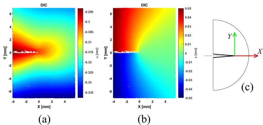
Metals 2020, 10, 400                                                                                                                 6 of 13

        Table 3. Values of the SIFs obtained by critical fracture load and by fitting the displacement field.

                                                                         By Crack Tip Displacement
      Specimen             By Critical Fracture Load (PCR)                                                        DIC vs. PCR
                                                                                Field (DIC)
     Configuration                √                   √                        √                √
                           KI (MPa m)         KII (MPa m)               KI (MPa m)      KII (MPa m)         ∆ KI (%)        ∆ KII (%)
     SM-0-42-42-1               32.1                 0.0                    58.3              1.2               81               -
     SM-0-42-42-2               30.4                 0.0                    56.1              2.9               85               -
     SM-0-42-42-3               33.7                 0.0                    60.5              2.3               80               -
     AM-0-42-42-1               42.5                 0.0                    73.5              0.2               73               -
     AM-0-42-42-2               44.9                 0.0                    76.4              0.1               70               -
     AM-0-42-42-3               46.6                 0.0                    75.2              0.2               61               -
    AM-10-42-42-1               44.4                16.5                    70.5             20.5               59              25
    AM-10-42-42-2               44.6                16.5                    66.2             18.3               49              11
    AM-10-42-42-3               45.1                16.7                    70.2             18.3               56              10
    AM-10-42-18-1               33.7                36.1                    43.7             42.2               30              17
    AM-10-42-18-2               36.3                38.8                    39.2             43.4                8              12
    AM-10-42-18-3               34.4                36.9                    44.2             45.7               28              24
    AM-10-42-10.2-1             15.3                83.5                    14.9             77.1               −2              −8
    AM-10-42-10.2-2             13.6                74.2                    14.4             75.5                5               2
    AM-10-42-10.2-3             14.2                79.4                    14.9             80.8                5               2

3.2. Evaluation of Stress Intensity Factors by the DIC Full Displacement Field
     To model the displacement near the crack tip, the Williams’ asymptotic formulation [25] was
exploited. The u and v are the displacement along the crack axis (x-axis) and along an axis perpendicular
to the former and contained in the crack plane (y-axis). Figure 4 show the u and v displacement field
measured by the DIC and postprocessed in MATLAB ® R2019b (MathWorks Inc., Natick, MA, USA)
along with the frame of reference used, with the origin located into the crack tip and the axis oriented
as shown in Figure
             Metals 2020,4c.
                         10, x FOR PEER REVIEW                                          6 of 14

      Figure 4. (a) Figure
                     x-displacement        (u) and
                           4. (a) x-displacement     (b) (b)
                                                 (u) and  y-displacement
                                                             y-displacement (v)(v)   of AM-0-42-42-1
                                                                                 of the the AM-0-42-42-1        specimen
                                                                                                      specimen obtained by obtained by
                    the DIC (digital image correlation). (c) Position and orientation of the frame of reference used.
      the DIC (digital   image correlation). (c) Position and orientation of the frame of reference used.
                       For Mode I, u and v are computed as functions of the polar coordinates (r, θ), according to the
     For Mode     I, useries
              infinite andofvEquations (3) and (4).as functions of the polar coordinates (r, θ), according to the
                              are computed
infinite series of Equations (3) and (4).                               ( − 4)
                                       =               +       + (−1)            −                                   (3)
                                             2             2                 2       2   2
                                       ∞      n
                                                                      nθ ( −n4) (n − 4)θ
                                                  (                                     )
                                             r         n
                                       X      2

                                                                n
                                uI =   =
                                                an κ−+ − (−1)
                                                            ( )
                                                          + −1 cos  + 2
                                                                         − cos                                       (4)                 (3)
                                             2µ
                                              2      2 2         2   2      22      2
                                       n=1
                     For Mode II, u and v aren computed   as functions of the polar coordinates (r, θ), according to the
                                        ∞
                                                                             nθ n (n − 4)θ
                                                   (                                                   )
                infinite series of Equationsr(5)           n
                                       X      2 and (6).

                                                                      n
                                vI =             an κ − − (−1) sin                + sin                                                  (4)
                                             2µ            2                  2 ( 2− 4)         2
                                       n
                                      =− = 1             + − (−1)           −                                      (5)
                                               2          2               2   2        2
     For Mode II, u and v are computed as functions of the polar coordinates (r, θ), according to the
infinite series of Equations (5)= and (6). − + (−1)         ( − 4)
                                                      +                             (6)
                                             2             2                 2       2   2

                where µ = E/(2 + 2ν) is the shear modulus and κ = (3−ν)/(1 + ν) for plane stress and κ = 3−4ν for plane
                strain condition; an and bn are the model parameters. In this analysis, the specimen was considered
                subjected to plane stress condition, which is an assumption justified by the specimen geometry and
                loading conditions [20].
                     For mixed modes, the displacement fields can be computed as the superimposition of the
                displacement of Mode I and Mode II, as shown in Equations (7) and (8).
                                                           =    +                                                 (7)
                                                                =   +                                                (8)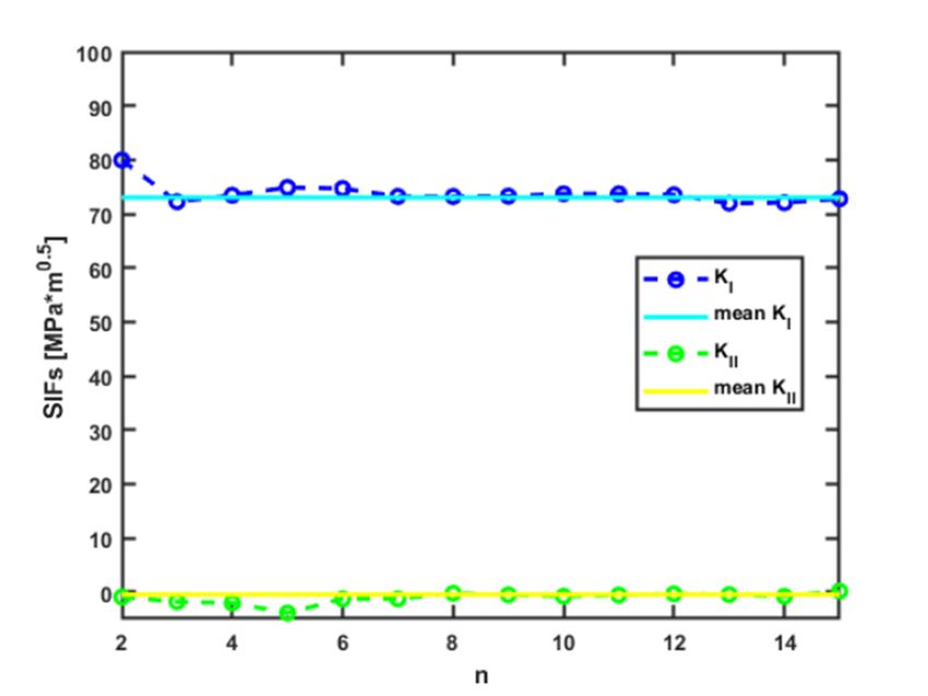
Metals 2020, 10, 400                                                                                       7 of 13

                                 ∞  n
                                                        nθ n (n − 4)θ
                                        (                            )
                                   r2       n
                                 X
                                                   n
                         uII = −      bn κ + − (−1) sin    − cos                                              (5)
                                   2µ       2            2  2    2
                                  n=1

                                 ∞  n
                                                         nθ n (n − 4)θ
                                        (                             )
                                   r2       n
                                 X
                         vII =        bn κ − + (−1)n cos    + cos                                             (6)
                                   2µ       2             2  2    2
                                 n=1

where µ = E/(2 + 2ν) is the shear modulus and κ = (3−ν)/(1 + ν) for plane stress and κ = 3−4ν for plane
strain condition; an and bn are the model parameters. In this analysis, the specimen was considered
subjected to plane stress condition, which is an assumption justified by the specimen geometry and
loading conditions [20].
     For mixed modes, the displacement fields can be computed as the superimposition of the
displacement of Mode I and Mode II, as shown in Equations (7) and (8).

                                                   u = uI + uII                                               (7)

                                                   v = vI + vII                                               (8)

    The values of KI and KII are related to the value of the Williams model parameters as shown in
Equations (9) and (10).                             √
                                            KI = a1 2π                                         (9)
                                                     √
                                           KII = −b1 2π                                       (10)

      To perform the fitting, not only the parameters a = a1 , . . . , an and b = b1 , . . . , bn were considered,
but also four additional parameters were accounted to compensate rigids motions, which is an
approach used also in [19,20]. In particular, the three translations and the rotation around the z-axis
(perpendicular to the crack plane) were considered. As explained in [19], this approach allows one
to tackle situations in which the material exhibits small-scale plastic deformation, but makes the
fitting problem non-linear in the fitting parameters, because of the x and y translations x0 and y0 ,
are embedded in the calculus of the polar coordinates (r, θ) as shown in Equations (11) and (12).
This approach was particularly useful in the case of the SM specimens, because the fact that they were
pre-cracked would have made difficult a precise manual identification of the crack tip.
                                              q
                                         r=       ( x − x0 ) 2 + ( y − y0 ) 2                                (11)

                                                             y − y0
                                              θ = arctg(            )                                        (12)
                                                             x − x0
     The fitting was performed by a code developed in MATLAB ® by the authors, which exploits the
function “lsqcurvefit”. The code is made publicly available at the link provided in the “Supplementary
Materials” section. To perform the fitting, it was decided to utilize the y-displacement v, since is the
one generally used to determinate the SIFs for Mode I, and for mixed mode problems the dominant
displacement component for the crack cannot be known in advance [19].
     A plasticization radius of 0.51 and 0.83 mm was calculated for Mode I and II respectively,
according to the following equations: rp = 1/π(KI /σYS )2 and rpII = 3/(2π)(KII /σYS )2 where σYS is
the yield strength of the material reported in Table 1 and KI and KII are the SIFs determined by the
DIC method reported in Table 3 (considering the AM specimens in the case of Mode I and Mode II).
However, we decided to only exclude the DIC data within 0.20 mm from the crack face (for every mode
mixity), because they were very noisy and not reliable there, but to keep all the other data in the fitting.
Indeed, the employed fitting method, in which the crack tip position is treated as an unknow quantity,
can effectively provide the SIFs for small-scale yielding, as it was shown by Yoneyama et al. [19].
These assumptions are furthermore justified by the fact that the specimen material exhibits a mainly
fragile behavior, as reported in [26].
[19].
A plasticization radius of 0.51 and 0.83 mm was calculated for Mode I and II respectively,
2 2
according to the following equations: = 1⁄π ( ⁄ ) and = 3⁄(2π) ( ⁄ ) where
is the yield strength of the material reported in Table 1 and and are the SIFs determined by
the DIC method reported in Table 3 (considering the AM specimens in the case of Mode I and Mode
II). However, we decided to only exclude the DIC data within 0.20 mm from the crack face (for every
Metals 2020, 10, 400
mode mixity), because they were very noisy and not reliable there, but to keep all the other data in 8 of 13
the fitting. Indeed, the employed fitting method, in which the crack tip position is treated as an
unknow quantity, can effectively provide the SIFs for small-scale yielding, as it was shown by
Yoneyama
Figure 5 shows theetSIFs
al. [19]. Theseobtained
values assumptions byare
thefurthermore
fitting forjustified by the
different fact that
values of the specimen of terms of
n (number
material exhibits a mainly fragile behavior, as reported in [26].
the Willams’ expansion) rising from 2 to 15. The higher order terms of the series are fundamental for a
Figure 5 shows the SIFs values obtained by the fitting for different values of n (number of terms
better estimation of theof the displacement
Willams’ expansion) risingin wider
from 2 to 15.areas nearorder
The higher to the
termscrack
of thetip,
seriesin
arewhich the effect of the
fundamental
singular termsforisalessbetterevident.
estimationIn of the displacement
general, it was in noted
wider areas
thatnear to the
after crack tip,
about 7–8interms
which thetheeffect of converges,
series
the singular terms is less evident. In general, it was noted that after about 7–8 terms the series
and for this reason the final SIFs values were obtained by computing the average
converges, and for this reason the final SIFs values were obtained by computing the average in the
in the range between
8th and 15th terms.
range between 8th and 15th terms.
Figure 5. Stress intensity
Figure factors
5. Stress forfactors
intensity values forof n ranging
values fromfrom
of n ranging 2 to 15
2 toin
15the case
in the ofof
case AM-0-42-42-1
AM-0-42-42-1 specimen.
specimen.
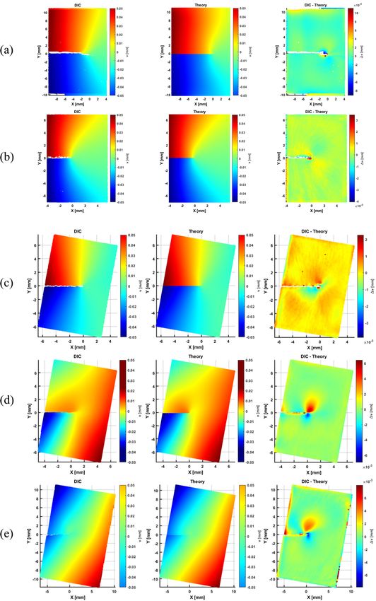
In Figure 6a comparison between the v-displacements field measured by the DIC and the one
In Figure 6a comparison between the v-displacements field measured by the DIC and the one
fitted by the Williams’ model model
fitted by the Williams’ is shown
is shownforforvarious combinations
various combinations of Mode ofI and
Mode
II. AsIexpected,
and II.the
As expected,
the v-displacements field for
v-displacements Mode
field I (opening)
for Mode I (opening)isis symmetric with
symmetric with respect
respect to the
to the crack crack
axis, axis,
whereas for whereas for
mixed mode I-II and Mode II (sliding) the symmetry axis rotates due the shear deformation. In the
mixed mode I-II and Mode II (sliding) the symmetry axis rotates due the shear deformation. In the third
third column of Figure 6, the difference between the displacement fitted by the theoretical model and
column of Figure 6, the difference between the displacement fitted by the theoretical model and the one
measured by the DIC is plotted. By ranging from Mode I to Mode II, the area where the linear elastic
model overestimates the experimental displacement field grows. Figure 7 shows the u-displacement
for the AM-10-42-10.2 specimen, which is more significative than the v-displacement since Mode II
is predominant. Indeed, a higher absolute error is shown for the u-displacement compared to the
v-displacement, being higher the u values for Mode II with respect to the v values.
The SIFs obtained by the full displacement field (DIC) and critical fracture load (PCR) are listed in
Table 3. As expected, the KIC measured for the specimens with the sintered crack-like notch (AM),
compared to the pre-cracked one (SM), is overestimated of about 40% and 30% for the PCR and the DIC
method, respectively. The reason is attributed to the larger radius of the crack-like notch compared to
the one, significantly smaller, of the case of the pre-cracked specimens. However, with this specimen
geometry, the pre-crack could be induced without having a deviation from its principal axis only for
Mode I, and for this reason mixed mode SIFs were investigated only with crack-like notch directly
induced by the AM process. For Mode I, an overestimation of about 70% of the DIC results with
respect to conventional PCR method can be observed. Going from Mode I to Mode II, this discrepancy
becomes negligible.Metals 2020, 10, 400 9 of 13
Metals 2020, 10, x FOR PEER REVIEW 9 of 14
Figure 6. Comparison
Figure 6. Comparison the v-displacements
betweenbetween the v-displacementsfield measured
field measured by by the and
the DIC DICtheand
one the
fittedone
by fitted by the
the Williams’ model for various specimens and loading condition: (a) SM-0-42-42
Williams’ model for various specimens and loading condition: (a) SM-0-42-42 (Mode I, pre-cracked); (Mode I, pre-
cracked); (b) AM-0-42-42 (Mode I); (c) AM-10-42-42 (mixed mode I-II); (d) AM-10-42-18 (mixed mode
(b) AM-0-42-42 (Mode I); (c) AM-10-42-42 (mixed mode I-II); (d) AM-10-42-18 (mixed mode I-II);
I-II); (e) AM-10-42-10.2 (Mode II).
Metals 2020, 10, x FOR PEER REVIEW 10 of 14
(e) AM-10-42-10.2 (Mode II).
Figure 7. u-displacements field measured
Figure 7. u-displacements bybythe
field measured theDIC and
DIC and thethe
oneone
fittedfitted by the Williams’
by the Williams’ model in themodel in the
case of the specimen AM-10-42-10.2
case of the specimen AM-10-42-10.2 (Mode II). (Mode II).
The SIFs obtained by the full displacement field (DIC) and critical fracture load (PCR) are listed
in Table 3. As expected, the KIC measured for the specimens with the sintered crack-like notch (AM),
compared to the pre-cracked one (SM), is overestimated of about 40% and 30% for the PCR and the
DIC method, respectively. The reason is attributed to the larger radius of the crack-like notch
compared to the one, significantly smaller, of the case of the pre-cracked specimens. However, with
this specimen geometry, the pre-crack could be induced without having a deviation from its principal
axis only for Mode I, and for this reason mixed mode SIFs were investigated only with crack-likeMetals 2020, 10, 400 10 of 13
3.3. Generalized Mixed-Mode Local Stress Criterium
To study the overall mixed-mode fracture toughness behavior of the sintered maraging steel,
the SIFs previously obtained were plotted on the graph KI –KII , normalized to KIC , which is the critical
SIF obtained for Mode I. As a multiaxial fracture model, the local stress criterium (LS), proposed by
Yongming Liu in [27] was exploited. Classical criteria based on maximum tangential stress, as the
generalized maximum tangential stress one (GMTS) [28], can only predict fracture toughness
Metals 2020, 10, x FOR PEER REVIEW 11 of 14
of brittle
materials. On the other hand, a major advantage of the LS criterium is that it can be applied to different
SIF obtained for Mode I. As a multiaxial fracture model, the local stress criterium (LS), proposed by
materials (brittle and ductile), which experience either shear or tensile dominated crack propagation.
Yongming Liu in [27] was exploited. Classical criteria based on maximum tangential stress, as the
Therefore, thisgeneralized
model can be suitable
maximum for the
tangential strong,
stress but at
one (GMTS) thecan
[28], same
only time
predictductile,
fracture maraging
toughness ofsteel. The LS
mixed mode criterium is described by Equation (13), with s equal to KIIC /KIC . The
brittle materials. On the other hand, a major advantage of the LS criterium is that it can be applied
material to parameter
different materials (brittle and ductile), which experience either shear or tensile dominated crack
s is related to the material ductility and affects the critical plane orientation. If the parameter s is higher
propagation. Therefore, this model can be suitable for the strong, but at the same time ductile,
than 1, as in this
maraging A =The
case,steel. 9 (s 2 = s,criterium
mixedBmode
LS −1), Υ = 0. isThe equation
described 13 represents
by Equation (13), with s the
equalimplicit
to KIIC/KIC.curve of the
LS criterium, Theand material parameter s issrelated
the coefficient can beto the material ductility
determined and affects the
numerically bycritical plane
fitting theorientation.
experimental SIFs
If the parameter s is higher than 1, as in this case, A = 9 (s2−1), B = s, Υ = 0. The equation 13 represents
normalized tothe the K .
IC curve of the LS criterium, and the coefficient s can be determined numerically by fitting
implicit
the experimental SIFs normalized
r to the KIC.
k 2 k 2 2
1
kIC + k 2S + A kkH = B
+IC + IC =
KI
k 1 = 2 ( 1 + cos 2α ) + K 2 sin 2α (13)
2K
k2 = − 2=I sin (12α
+ cos
+2KII) +cossin
2α2 ; α = β + γ; β = 21 arctg KIII (13)
K
where :
=H
k − =sin32I + cos 2 ; = + ; = arctg
where:
K
=
As can be observed in Figure
As can be observed 8, the
in Figure LS LS
8, the criterium
criterium isisable
able tothe
to fit fitSIFs
the(ofSIFs (of specimens)
the AM the AM specimens)
obtained withobtained
both thewithPCR and
both the the
PCR DIC
and methods.
the DIC methods.
Figure 8. Fitting
Figureof
8. the local
Fitting of thestress criterium
local stress criteriumon
on the experimental
the experimental data
data of of the
the AM AM specimens.
specimens.
4. Discussion4. Discussion
Pure and mixed mode I-II SIFs were evaluated for ASCB specimens of maraging steel produced
Pure andbymixed mode
additive SLS I-II SIFsSIFs
process. were of evaluated
44.7 MPa mfor ASCB
0.5 and 79.1 specimens
MPa m0.5 wereof obtained
maraging steel
with PCRproduced by
additive SLS process.
methodology SIFs of 44.7
for Mode MPa
I and Mode 0.5respectively.
mII, and 79.1 MPa m0.5 were obtained with PCR methodology
The feasibility of inducing crack-like notches directly during the additive manufacturing (AM)
for Mode I and Mode II, respectively.
process was investigated and compared with the classical subtractive one (SM), for Mode I. The AM
The feasibility of inducing
method could be used to crack-like notchesinternal
induce in the specimen directly during
crack-like thewith
notches additive manufacturing
any angle and shape (AM)
process was investigated and compared
and study three-dimensional with
fracture the classical
mechanics subtractive
problems, which would onenot(SM), for Mode
be feasible with I. The AM
method couldconventional
be used methods.
to induce Micrograph analysis shows that a notch with a slightly sharp tip with a radius
in the specimen internal crack-like notches with any angle and
smaller than 100 μm can be obtained by the AM technique. As expected, an overestimation of about
shape and study three-dimensional
30–40% of the SIFs was measured fracture mechanics
for the crack-like notchproblems,
produced bywhich would
AM technique, not betofeasible with
compared
conventional methods. Micrograph
the fatigue loading pre-crackedanalysis shows
one. Indeed, beingthat a notch sharper
the pre-crack with athan
slightly sharpone,
the sintered tipthe
with a radius
stress concentration at the tip is higher, and therefore the specimen would fail with a lower load,
smaller than 100 µm can be obtained by the AM technique. As expected, an overestimation of about
30–40% of the SIFs was measured for the crack-like notch produced by AM technique, compared to
the fatigue loading pre-cracked one. Indeed, being the pre-crack sharper than the sintered one,
the stress concentration at the tip is higher, and therefore the specimen would fail with a lower load,Metals 2020, 10, 400 11 of 13
which corresponds to a lower SIF. Comparing the obtained results, for maraging steel, with the one
reported by the author in [3], for Nylon polymer, the discrepancy between the crack-like notch induced
by AM and SM technique is higher (30–40 % vs. 2–4 %). This can be explained by the different ductility
of the two studied materials. Indeed, the polymer, being more ductile, is less sensible to the sharpness
of the notch.
Two different methods for evaluating the SIFs were compared: the classical one based on the
critical load (PCR) and a less conventional one based on fitting of the Williams’ model on the full field
displacement measurement at the crack tip (DIC). This latter method could be used for non-destructive
analysis by the DIC of the crack status in three dimensional structures were the stress state is difficult
to be predicted. For Mode I, an overestimation of about 70% of the DIC results with respect to the
conventional PCR method can be observed. While going from Mode I to Mode II this discrepancy
become negligible.
It is well known in literature [29] (p. 76) that the Mode I SIF depends on the three-dimensional
stress state at the crack tip. In particular, it is overestimated for thin specimens, which are in plane stress
condition, whereas it decreases for increasing specimen thickness until a plateau is reached at plane
strain state. Amr A. Abd-Elhady [30] conducted a three-dimensional finite element analysis on SCB
specimens in order to evaluate the SIF throughout the thickness for mixed mode I/II loading condition.
The Author observed that for Mode I, the geometry factor decreases moving from the mid-plane to the
outer surface of the specimen, in order to compensate for the higher apparent SIF due to the plane
stress condition. Conversely, for Mode II, the SIF is less dependent on the thickness and shows an
opposite trend with respect to Mode I. Hence, in our case, the overestimation of the Mode I SIFs via the
DIC can be attributed to the fact that the method evaluates it by exploiting the measured displacement
field on the outer surface, which is on plane stress condition. This phenomenon becomes less marked
varying from Mode I to Mode II according to the numerical results of Amr A. Abd-Elhady [30].
5. Conclusions
Mixed and Mode I and II SIFs were evaluated for maraging steel ASCB specimens produced by
the additive SLS process. A non-conventional method to induce crack-like notches directly during
the additive manufacturing process was proposed and validated on metal specimens. Two different
methods for evaluating the SIFs were compared: the classical one based on the critical load and a less
conventional one based on the fitting of the Williams’ model on the full field displacement measurement
at the crack tip, measured by a DIC system. Finally, the experimental results were described by the
mixed mode local stress criterium.
Supplementary Materials: The MATLAB® code used for the calculation of the DIC method is online at
http://www.mdpi.com/2075-4701/10/3/400/s1.
Author Contributions: Conceptualization, T.M.B. and G.M.; Funding acquisition, S.Ć.K.; Investigation,
I.C. and T.M.B.; Methodology, I.C. and T.M.B.; Sample production, J.J.T., S.Ć.K. and N.B.; Software, I.C.;
Supervision, G.M.; Visualization, N.B.; Writing—original draft, I.C. and T.M.B.; Writing—review & editing, T.M.B.
and G.M. All authors have read and agreed to the published version of the manuscript.
Funding: The research presented in this paper is part of the A_Madam Project, funded by the European Union’s
Horizon 2020 research and innovation program under the Marie Skłodowska-Curie action, grant agreement
No. 734455.
Acknowledgments: The authors would like to thank Nenad Drvar and Josip Kos from Topomatika
(Zagreb, Croatia), for the technical support on the DIC measurements. Two of the authors (N.B. and S.Ć.K.) would
like to acknowledge support of the Serbian Ministry of Education, Science and Technology Development.
Conflicts of Interest: The authors declare no conflict of interest.
References
1. Kruth, J.; Mercelis, P.; van Vaerenbergh, J.; Froyen, L.; Rombouts, M. Binding mechanisms in selective laser
sintering and selective laser melting. Rapid Prototyp. J. 2005, 11, 26–36. [CrossRef]Metals 2020, 10, 400 12 of 13
2. Zhang, W.; Melcher, R.; Travitzky, N.; Bordia, R.K.; Greil, P. Three-dimensional printing of complex-shaped
alumina/glass composites. Adv. Eng. Mater. 2009, 11, 1039–1043. [CrossRef]
3. Brugo, T.; Palazzetti, R.; Ciric-Kostic, S.; Yan, X.T.; Minak, G.; Zucchelli, A. Fracture Mechanics of laser
sintered cracked polyamide for a new method to induce cracks by additive manufacturing. Polym. Test.
2016, 50, 301–308. [CrossRef]
4. Williams, J.G.; Ewing, P.D. Fracture under complex stress—The angled crack problem. Int. J. Fract. Mech.
1972, 8, 441–446. [CrossRef]
5. Papadopoulos, G.A.; Poniridis, P.I. Crack initiation under biaxial loading with higher-order approximation.
Eng. Fract. Mech. 1989, 32, 351–360. [CrossRef]
6. Silva, A.L.L.; de Jesus, A.M.P.; Xavier, J.; Correia, J.A.F.O.; Fernandes, A.A. Combined analytical-numerical
methodologies for the evaluation of mixed-mode (I + II) fatigue crack growth rates in structural steels.
Eng. Fract. Mech. 2017, 185, 124–138. [CrossRef]
7. Aliha, M.R.M.; Ayatollahi, M.R. Brittle fracture evaluation of a fine grain cement mortar in combined
tensile-shear deformation. Fatigue Fract. Eng. Mater. Struct. 2009, 32, 987–994. [CrossRef]
8. Lim, I.L.; Johnston, I.W.; Choi, S.K.; Boland, J.N. Fracture testing of a soft rock with semi-circular specimens
under three-point bending. Part 2—Mixed-mode. Int. J. Rock Mech. Min. Sci. Geomech. Abstr. 1994, 31,
199–212. [CrossRef]
9. Ayatollahi, M.R.; Aliha, M.R.M.; Saghafi, H. An improved semi-circular bend specimen for investigating
mixed mode brittle fracture. Eng. Fract. Mech. 2011, 78, 110–123. [CrossRef]
10. Darban, H.; Haghpanahi, M.; Assadi, A. Determination of crack tip parameters for ascb specimen under
mixed mode loading using finite element method. Comput. Mater. Sci. 2011, 50, 1667–1674. [CrossRef]
11. Saghafi, H.; Monemian, S.A. New fracture toughness test covering mixed-mode conditions and positive and
negative t-stresses. Int. J. Fract. 2010, 165, 135–138. [CrossRef]
12. Saghafi, H.; Zucchelli, A.; Minak, G. Evaluating fracture behavior of brittle polymeric materials using an
IASCB specimen. Polym. Test. 2013, 32, 133–140. [CrossRef]
13. Moore, A.J.; Tyrer, J.R. The evaluation of fracture mechanics parameters from electronic speckle pattern
interferometric fringe patterns. Opt. Lasers Eng. 1993, 19, 325–336. [CrossRef]
14. Peters, H.W.; Ranson, F.W. Digital imaging techniques in experimental stress analysis. Opt. Eng. 1982, 21,
427–431.
15. McNeill, S.R.; Peters, W.H.; Sutton, M.A. Estimation of stress intensity factor by digital image correlation.
Eng. Fract. Mech. 1987, 28, 101–112. [CrossRef]
16. Muskhelishvili, N.I. Some Basic Problems of the Mathematical Theory of Elasticity, 4th ed.; Springer:
Berlin, Germany, 1977.
17. Nurse, A.D.; Patterson, E.A. Determination of predominantly mode II stress intensity factors from
isochromatic data. Fatigue Fract. Eng. Mater. Struct. 1993, 16, 1339–1354. [CrossRef]
18. Lopez-Crespo, P.; Shterenlikht, A.; Patterson, E.A.; Yates, J.R.; Withers, P.J. The stress intensity of mixed mode
cracks determined by digital image correlation. J. Strain Anal. Eng. Des. 2008, 43, 769–780. [CrossRef]
19. Yoneyama, S.; Ogawa, T.; Kobayashi, Y. Evaluating mixed-mode stress intensity factors from full-field
displacement fields obtained by optical methods. Eng. Fract. Mech. 2007, 74, 1399–1412. [CrossRef]
20. Yates, J.R.; Zanganeh, M.; Asquith, D.; Tai, Y.H. Quantifying Crack Tip Displacement Fields: T-Stress and
CTOA. In Proceedings of the Crack Paths, Vicenza, Italy, 23–25 September 2009.
21. Beretta, S.; Patriarca, L.; Rabbolini, S. Stress intensity factor calculation from displacement fields. Frat. ED
Integrità Strutt. 2017, 11, 269–276. [CrossRef]
22. Bonniot, T.; Doquet, V.; Mai, S.H. Determination of effective stress intensity factors under mixed-mode
from digital image correlation fields in presence of contact stresses and plasticity. Strain 2020, 56, e12332.
[CrossRef]
23. Croccolo, D.; de Agostinis, M.; Fini, S.; Olmi, G.; Vranic, A.; Ciric-Kostic, S. Influence of the build orientation
on the fatigue strength of eos maraging steel produced by additive metal machine: How the build direction
affects the fatigue strength of additive manufacturing processed parts. Fatigue Fract. Eng. Mater. Struct.
2016, 39, 637–647. [CrossRef]
24. Palanca, M.; Brugo, T.M.; Cristofolini, L. Use of digital image correlation to investigate the biomechanics of
the vertebra. J. Mech. Med. Biol. 2015, 15, 1540004. [CrossRef]Metals 2020, 10, 400 13 of 13
25. Williams, M.L. On the stress distribution at the base of a stationary crack. J. Appl. Mech. 1957, 24, 109–114.
[CrossRef]
26. Tan, C.; Zhou, K.; Ma, W.; Zhang, P.; Liu, M.; Kuang, T. Microstructural evolution, nanoprecipitation behavior
and mechanical properties of selective laser melted high-performance grade 300 maraging steel. Mater. Des.
2017, 134, 23–34. [CrossRef]
27. Liu, Y.; Mahadevan, S. Threshold stress intensity factor and crack growth rate prediction under mixed-mode
loading. Eng. Fract. Mech. 2007, 74, 332–345. [CrossRef]
28. Smith, D.J.; Ayatollahi, M.R.; Pavier, M.J. The role of t-stress in brittle fracture for linear elastic materials
under mixed-mode loading. Fatigue Fract. Eng. Mater. Struct. 2001, 24, 137–150. [CrossRef]
29. Anderson, T.L. Fracture Mechanics: Fundamentals and Applications, 3rd ed.; CRC Press, Taylor & Francis Group:
Boca Raton, FL, USA, 2005.
30. Abd-Elhady, A.A. Mixed mode I/II stress intensity factors through the thickness of disc type specimens.
Eng. Solid Mech. 2013, 1, 119–128. [CrossRef]
© 2020 by the authors. Licensee MDPI, Basel, Switzerland. This article is an open access
article distributed under the terms and conditions of the Creative Commons Attribution
(CC BY) license (http://creativecommons.org/licenses/by/4.0/).You can also read