Growing Cosine Unit: A Novel Oscillatory Activation Function That Can Speedup Training and Reduce Parameters in Convolutional Neural Networks
←
→
Page content transcription
If your browser does not render page correctly, please read the page content below

Growing Cosine Unit: A Novel Oscillatory Activation
                                         Function That Can Speedup Training and Reduce
                                          Parameters in Convolutional Neural Networks

                                                Mathew Mithra Noel                       Arunkumar L                    Advait Trivedi
                                            Vellore Institute of Technology      Vellore Institute of Technology     astrived@ncsu.edu
arXiv:2108.12943v2 [cs.LG] 4 Sep 2021

                                            mathew.mithra@gmail.com                  arunk609@gmail.com

                                                                                    Praneet Dutta
                                                                              praneetd@alumni.cmu.edu

                                                                                      Abstract

                                                  Convolution neural networks have been successful in solving many socially im-
                                                  portant and economically significant problems. Their ability to learn complex
                                                  high-dimensional functions hierarchically can be attributed to the use of nonlinear
                                                  activation functions. A key discovery that made training deep networks feasible
                                                  was the adoption of the Rectified Linear Unit (ReLU) activation function to allevi-
                                                  ate the vanishing gradient problem caused by using saturating activation functions.
                                                  Since then many improved variants of the ReLU activation have been proposed.
                                                  However a majority of activation functions used today are non-oscillatory and
                                                  monotonically increasing due to their biological plausibility. This paper demon-
                                                  strates that oscillatory activation functions can improve gradient flow and reduce
                                                  network size. It is shown that oscillatory activation functions allow neurons to
                                                  switch classification (sign of output) within the interior of neuronal hyperplane
                                                  positive and negative half-spaces allowing complex decisions with fewer neurons.
                                                  A new oscillatory activation function C(z) = z · cos z that outperforms Sigmoids,
                                                  Swish, Mish and ReLU on a variety of architectures and benchmarks is presented.
                                                  This new activation function allows even single neurons to exhibit nonlinear deci-
                                                  sion boundaries. This paper presents a single neuron solution to the famous XOR
                                                  problem. Experimental results indicate that replacing the activation function in the
                                                  convolutional layers with C(z) significantly improves performance on CIFAR-10,
                                                  CIFAR-100 and Imagenette.

                                        1    Introduction
                                        The quintessential feature of deep convolutional neural networks is their ability to learn arbitrarily
                                        complex nonlinear mappings between high-dimensional input to a target output. This universal
                                        approximation feature is critically dependent on the nature of the activation function non-linearity
                                        used by each layer in the neural network. Training a neural network might be viewed as adjusting
                                        a set of parameters to scale, compress, dilate, combine and compose simple nonlinear activation
                                        functions to approximate a complex nonlinear target function.
                                        The property of activation functions to be nonlinear is essential, since the composition of any finite
                                        number of linear functions is equivalent to a single linear function. Hence, the resultant network
                                        composed of purely linear neurons is equivalent to a single linear layer network limited to solving
                                        linearly separable problems. Despite the critical importance of the nature of the activation function
                                        in determining the performance of neural networks, simple monotonic non decreasing nonlinear

                                        Preprint. Under review.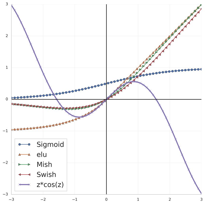
activation functions are universally used. In this work, we explore the effects of using oscillatory
nonlinear activation functions in deep neural networks.
In the past, sigmoidal [10]saturating activation functions were widely used due to their property
of approximating the step or signum function while being differentiable. The outputs of s-shaped
saturating activations have the important property of being interpretable as a binary yes/no decision
and hence are useful. However, deep neural networks composed of purely sigmoidal activation
functions are hard to train, due to the vanishing gradient phenomenon which arises when saturating
activation functions are used. The adoption of non-saturating and non-sigmoidal Recti-Linear Unit
(ReLU) [1] activation function to alleviate the vanishing gradient problem is considered a milestone
in the evolution of deep neural networks.
During training, the parameters are continually updated in the direction of the negative gradient.
Hence small gradients lead to stagnation in learning and slow parameter updates. The derivative
of sigmoidal activation functions with respect to the input input is small outside a small closed
interval around zero (usually [-5 , 5]). In particular exp(−5) < 0.01 and hence activation functions
composed purely of exponentials, such as logistic-sigmoid and tan-sigmoid will saturate outside this
narrow range.
Furthermore, in uni-polar activation functions (functions that take purely non-negative values like
logistic-sigmoid), the outputs of a layer can get combined to form large positive values leading to
the saturation of neurons in the next layer. Thus, activation functions that do not shift the mean of
the input towards positive or negative values (such as tanh(z)) reduce saturation of succeeding layers
and hence perform better.
In the past a wide variety of activation functions have been explored [7], which was the inspiration
behind the Swish activation function. [11]. Past research indicates that activation functions that
have larger derivative values for a wider set of input values perform better. In particular the use of
the ReLU like activation functions result in faster training compared to saturating sigmoidal type
activation functions because these activation functions do not saturate for a wider range of inputs.
Some drawbacks of ReLU like activation functions:

       • The derivative of the loss function J with respect to the weight matrix W k of layer k is
          ∂J
         ∂W k
               = δ k (ak−1 )T . Thus if ak−1 is small then this derivative is also small, the weights are
         not updated and learning stagnates.
       • Bias Shift: There is a positive bias in the network for subsequent layers, as the mean
         activation is always greater than zero. Since the outputs of all ReLU units are non-negative
         the outputs can combine to produce very large positive inputs to subsequent layers farther
         away from the input leading to possible saturation and numerical accuracy issues.
                                                    ∂J
       • The delta for a particular layer is δ k = ∂z           k+1 T k+1
                                                                            ) g 0 (z k ), where g 0 (z k )
                                                                              J
                                                      k = ((W       ) δ
         is the derivative of the activation function. So ReLU like activation functions that have
         zero or small derivative for negative values result is small δ k values leading to stagnation
         in learning.

Variants of ReLU: SELU [5], ELU [2] have been successful to an extent in mitigating these short-
comings. Swish [12] and Mish [9] represent a new class of non-monotonic functions that offer
promising results across different benchmarks.
Despite the popularity of a wide variety of activation functions and neural network architectures,
all networks suffer from a fundamental limitation in that individual neurons can exhibit only linear
decision boundaries. Multilayer neural networks with nonlinear activations are needed to achieve
nonlinear decision boundaries. This paper explores proposes a new oscillatory activation function
that allows individual neurons to exhibit nonlinear decision boundaries thus removing a fundamental
limitation of neural networks.
In brief, the contributions of this work are:

       • A new activation function, Growing Cosine Unit (GCU) defined by C(z) = z · cos(z)
         has been proposed. The advantages of using oscillatory activation functions to improve
         gradient flow and alleviate the vanish gradient problem has been demonstrated.

                                                    2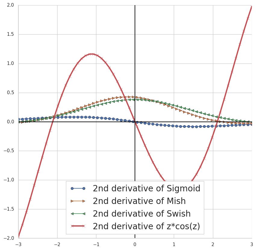
• A solution to the classic XOR problem has been demonstrated by successfully training a
         single neuron with the C(z) = z · cos(z) activation function to learn this function.

       • Two theorems that characterize the limitation of certain class of activation functions are
         presented.

       • A comparison of the proposed GCU activation with popular activation functions on a va-
         riety of benchmark datasets is presented in Section 4. These experimental results clearly
         indicate that the GCU activation is computationally cheaper than Swish and Mish. The
         GCU activation also reduces training time and allows classification problems to be solved
         with smaller networks.

2     Oscillatory Activation functions

This paper explores the potential performance benefits and effects of using oscillatory activation
functions in neural networks. In the past oscillatory and non-monotonic activation functions have
been largely ignored.
In our study, certain Oscillatory activation functions are shown to possess the following advantages:

       • Alleviate the vanishing gradient problem. These functions have non-zero derivatives
         throughout their domain except at isolated points.

       • Improved performance for compact network architectures.

       • Computationally cheaper than the state-of-the-art Swish and Mish activation functions.

2.1   Learning the XOR function using a single neuron

The famous XOR problem is task of training a neural network to learn the XOR gate function. It was
first pointed out by Papert and Minsky [8] that a single neuron cannot learn the XOR function since
a single hyperplane (line in this case) cannot separate the output classes for this function definition.
This fundamental limitation of single neurons (or single layer networks) lead to pessimistic predic-
tions for the future of neural network research and was responsible for a brief hiatus in the history
of AI. In the following section, we show that this issue does not apply to neurons with oscillatory
activation function (like GCU).
The XOR problem is the task of learning the following dataset:

                               −1           1          −1         1
                      D=     (    , −1), (    , 1), (     , 1), (    , −1)                          (1)
                               −1          −1          1          1

Figure 1: The XOR problem involves the task of learning the XOR function with the smallest
network. The red dots must be classified as positive (1) and the black dots must be classified as
negative (-1). A single line (hyperplane) cannot separate the two classes.

                                                   3
Figure 2: Two solutions to the XOR problem learnt by a single neuron using the GCU activation
function. Points in yellow were assigned a class label of +1 and points in blue were assigned a class
label of -1 by a single GCU neuron.
Figure 3: A single neuron solution to the XOR problem learnt by using a simple oscillatory poly-
3
nomial activation function Pc (z) = z − z2 . Points in yellow were assigned a class label of +1 and
points in blue were assigned a class label of -1 by a single neuron using the polynomial activation.
Figure 4: A single neuron solution to the XOR problem. A single neuron with the GCU activation
function is capable of learning the XOR dataset shown in (1) exactly. The signum function at the
output is used to map output values to ±1.
The XOR problem was solved by using a single neuron with oscillatory activation functions, mean-
square loss and simple Stochastic Gradient Descent (SGD). A learning rate of α = 0.01 and the
SGD update rule ∆w = α(y − g(z))g 0 (z)x, z = wT x + b was used. The initial weight vector
was initialized with uniform random numbers in the interval [0 , 1].
The XOR function was successfully learned by a single neuron with the activation functions g(z)
3
chosen to be g(z) = C(z) = z · cos(z) and g(z) = Pc (z) = z − z2 respectively. The target y for
each input was taken as the class label namely 1 or -1. After training the output of the neuron is
mapped to the class label in the usual manner. That is we assign positive outputs a label of +1 and
negative outputs a label of -1. This can be done simply by defining the class label Class(x) for each
input x to be Class(x) = sign(g(wT x + b)). Where the signum function is defined as
1 if z > 0
sign (z) = −1 if z < 0
0 if z = 0
Definition 1: The decision boundary of a single neuron is the set B = {x ∈ Rn : g(wT x + b) = 0}.
Where g is the activation function.
4
That is the boundary is the set of inputs that elicit an output of zero from the neuron. Inputs cor-
responding to positive outputs are assigned the positive class and inputs corresponding to negative
outputs are assigned the negative class (in accordance with Class(x) = sign(g(wT x + b))) as
already discussed.

It is clear from Definition 1 that the decision boundary for any neuron that uses an activation function
satisfying the condition
                                           g(z) = 0 ⇐⇒ z = 0
is
                                             z = wT x + b = 0
In other words the decision boundary is a single hyperplane (B = H).

However if g is an oscillatory function like C(z) = z cos z, the decision boundary is the set {x ∈
Rn : GCU(wT x + b) = 0} and consists of infinitely many hyperplanes in the input space, since
C(z) has infinitely many roots. In particular the decision boundary with the GCU activation is a set
of uniformly spaced parallel hyperplanes wT x + b = π2 + nπ. Thus the input space is divided into
parallel strips separated by the hyperplanes and point in adjacent strips are assigned different classes
alternately. These parallel strips can be seen in the solution to the XOR problem (Fig. 4).

2.2   Characterization of Activation Functions

In the following, we prove that no single neuron with a strictly monotone activation function can
learn the XOR function.
We adopt the following notation: The output (activation) of a single neuron is given by a = g(wT x+
b), where g is the activation function. The hyperplane boundary associated with a neuron is the set
of points:
                                    H = {x ∈ Rn : wT x + b = 0}
The positive and negative half spaces are similarly defined to be:
                                  H− = {x ∈ Rn : wT x + b < 0}
                                   H+ = {x ∈ Rn : wT x + b > 0}
Any hyperplane divides the input space Rn into 3 connected regions: the positive half-space H+ ,
the negative half-space H− and an affine-space H. The weight vector w points into the positive
half-space H+ .
The distance between a point x and the hyperplane decision boundary H is given by:
                                                    |wT x + b|
                                        d(x, H) =
                                                      kwk
.
Proposition 1: Consider a single neuron with weight vector w and bias b using an activation function
that is monotonically strictly increasing with g(0) = 0. The class label assigned to an input x by
this neuron is defined to be C(x) = sign(wT x + b). If a point x1 assigned to a particular class is
at a distance d1 from the hyperplane H = {x ∈ Rn : wT x + b = 0}, then any other point x2 at a
distance d2 > d1 in the same halfspace as x1 will be assigned to the same class by this neuron.

Proof:
Case 1: Consider the case where x1 ∈ H+ AND x2 ∈ H+
By assumption, z1 = wT x1 + b > 0 AND z2 = wT x2 + b > 0. Also d1 < d2
Using the formula for d(x,H):

                                      |wT x1 + b|   |wT x2 + b|
                                                  <
                                         kwk           kwk

                                                   5
wT x1 + b   wT x 2 + b
                                                 <
                                         kwk         kwk

                                        wT x1 + b < wT x2 + b

                                                z1 < z2

0 < z1 by assumption, thus 0 < z1 < z2 .
Since g is strictly increasing and g(0) = 0 : 0 < g(z1 ) < g(z2 )

                                               g(z2 ) > 0

                         Class(x2 ) = sign(wT x2 + b) = sign(g(z2 )) = 1
Thus x2 ∈ H+ and hence x2 belongs to the same class as x1 .
Case 2: Consider the case where x1 ∈ H− AND x2 ∈ H−
By assumption, z1 = wT x1 + b < 0 AND z2 = wT x2 + b < 0. Also d1 < d2
Using the formula for d(x,H):

                                      |wT x1 + b|   |wT x2 + b|
                                                  <
                                         kwk           kwk

                                   −(wT x1 + b)   −(wT x2 + b)
                                                <
                                      kwk            kwk

                                        wT x1 + b > wT x2 + b

                                                z1 > z2

0 > z1 by assumption, thus 0 > z1 > z2 . Since g is strictly increasing and g(0) = 0 : 0 > g(z1 ) >
g(z2 )

                                               0 > g(z2 )

                        Class(x2 ) = sign(wT x2 + b) = sign(g(z2 )) = −1
Thus x2 ∈ H− and hence x2 belongs to the same class as x1 .
Thus it is clear from Proposition 1, that if a point is assigned a particular class, other points further
away from the boundary are automatically assigned the same class by strictly monotonic activation
functions. However oscillatory activation functions are not subject to this limitation,hence can learn
the XOR classification with a single neuron.

Definition 2: A function f : X → R is said to be sign equivalent to a function g : X → R iff
sign(f (x)) = sign(g(x)) for all x ∈ X.

It is clear that sign equivalence is actually an Equivalence relation on the set of all real-valued
functions on a set. Further we note that the set of functions G = {f : R → R : f (0) = 0} is a
vector space. Also the subset of functions of G that are sign equivalent to I(z) = z form a convex
cone in G.

                                                   6
Proposition 2: Consider a single neuron that uses an activation function that is sign equivalent to
the identity function I(z) = z, that is sign(g(z)) = sign(z). If x1 , x2 ∈ H+ , then Class(x1 ) =
Class(x2 ) = 1 and if x1 , x2 ∈ H− , then Class(x1 ) = Class(x2 ) = −1.

Proof:
Case 1: Let sign(g(z)) = sign(z) AND x1 , x2 ∈ H+

⇒ z1 = wT x1 + b > 0 AND z2 = wT x2 + b > 0

⇒ Class(x1 ) = sign(g(z1 )) = sign(z1 ) = 1 AND Class(x2 ) = sign(g(z2 )) = sign(z2 ) = 1

Thus x1 and x2 belong to the same class.

Case 2: Let sign(g(z)) = sign(z) AND x1 , x2 ∈ H−

⇒ z1 = wT x1 + b < 0 AND z2 = wT x2 + b < 0

⇒ Class(x1 ) = sign(g(z1 )) = sign(z1 ) = −1 AND Class(x2 ) = sign(g(z2 )) = sign(z2 ) =
−1

Thus x1 and x2 belong to the same class.
From Proposition 2 it is clear that a single neuron using the Swish activation function cannot solve
the XOR problem.

                                  z
The Swish activation S(z) =   1+exp(−z)
                                                   1
It is clear that sign(S(z)) = sign(z) (since   1+exp(−z)   > 0).

Similarly a single neuron using the Mish activation function cannot solve the XOR problem. The

Mish activation M (z) = z tanh(log(1 + exp(z))), It is clear that sign(M (z)) = sign(z) (since

tanh(log(1 + exp(z))) > 0).

Based on propositions 1 and 2, single neurons that use monotonic activation functions and activation
functions that are are sign equivalent to I(z) = z cannot solve the XOR problem. To solve the XOR
problem with a single neuron we must search for an activation that violates both the above condi-
tions. In our work, the oscillatory function C(z) = z cos z that violates both the above conditions is
proposed and used to solve the XOR problem with a single neuron.

                                                  7
3 Comparison of Computational complexity for activation functions
(a)
(b) (c)
Figure 5: (a) Plot of GCU (z cos z) and other activation functions. The corresponding first (b) and
second (c) derivatives.
Fig. 5 compares the features of different activation functions. It is clear that C(z) and the other
activation functions are very close to I(z) = z for small values of z. This is desirable and has
a regularizing effect since the network behaves like a linear classifier when initialized with small
weights. During training the weights get updated and the nonlinear range of GCU is utilized as
needed. In particular a GCU network can serve as a linear classifier if necessary avoiding overfitting
effects. Also the GCU activation temporarily saturates close to its first maximum and minimum
values and mimics the behaviour of sigmoids. For larger inputs GCU oscillates and is an unbounded
function.
8Name Function
1
Logistic-sigmoid σ(z) = 1+exp (−z)
tan-sigmoid T (z) = tanh z = exp(z)−exp(−z)
exp(z)+exp(−z)
z if z > 0
Rectified Linear Unit (ReLU) R(z) =
0 if z < 0
z if z > 0
Leaky ReLU L(z) =
0.01z if z < 0
z
Swish S(z) = 1+exp (−z)
Mish M (z) = z tanh (log(1 + exp (z)))
Growing Cosine Unit (GCU) C(z) = z cos z
Table 1: A list of activation functions considered in this paper and their definitions.
Figure 6: Average time over 1000 independent runs. Where each run consisted of applying the
activation to a vector of length 106 with elements uniformly distributed in the interval [-5 , 5].
Table 1 shows that the proposed GCU activation function is computationally cheaper than Swish
and Mish activation functions. For example GCU uses one transcendental function call and one
multiplication whereas the Mish activation function uses 3 transcendental function calls and one
multiplication. It is also evident from Fig.6 that the proposed GCU activation is computationally
cheaper than the Swish and Mish activation functions.
4 Comparison of performance on benchmark datasets
4.1 Experimental set up
In the following a comparison of the CNN models with the proposed GCU activation on the CIFAR-
10 [6], CIFAR-100, and Imagenette [4] datasets is presented. Imagenette is a subset of ImageNet
[3], which consists of ten classes of easily recognized objects. The RMSprop optimizer [14] is used
with the categorical cross entropy loss function(softmax classification head). For computational rea-
sons, we were unable to test this on the full ImageNet, which remains a future tasks. Experiments on
CIFAR-10, CIFAR-100 were carried out with an initial learning, decay rate of 10−4 , 10−6 respec-
tively. For Imagenette, this was 10−6 , with no decay. The Xavier Uniform initializer instantiates the
weights of the kernel layers. The GCU activation is used only for the convolutional layers and not
for the dense layers, being computationally costlier than the ReLU activation.
9CONV. Layer Dense Layer Top - 1 Acc. % SD Acc. Loss SD Loss
ReLU ReLU 74.13 0.56 0.74 0.016
GCU ReLU 75.64 0.47 0.73 0.004
Swish Swish 71.74 0.48 0.82 0.014
Swish ReLU 71.70 1.05 0.84 0.016
Mish Mish 74.22 0.62 0.77 0.004
Mish ReLU 73.20 0.74 0.79 0.011
Table 2: Validation set accuracy of various activation functions on the CIFAR-10 dataset
CONV. Layer Dense Layer Top- 1 Acc. % SD Acc. Loss SD Loss
ReLU ReLU 41.29 0.43 2.31 0.016
GCU ReLU 43.42 0.36 2.23 0.004
Swish Swish 39.37 0.40 2.43 0.014
Swish ReLU 38.46 0.42 2.45 0.016
Mish Mish 41.13 0.36 2.33 0.004
Mish ReLU 39.83 0.37 2.39 0.011
Table 3: Validation set accuracy of various activation functions on the CIFAR-100 dataset
The results for each of these are reported over 5 runs, each of 25 epochs. We leverage a compact net-
work architecture for CIFAR-10,100, as detailed in the Appendix section. The architecture consists
of only 4 convolutional layers, followed by dense layers. For ImageNette, we utilize the VGG-16
backbone. [13].
For both architectures tested, we experiment with the choice of activation functions at two locations:
one for all of the convolutional layer and the other for the dense layers.
Convolution Layer Activation Dense Layer Top- 1 Acc. % SD Acc. Loss SD Loss
ReLU ReLU 60.28 0.60 1.21 0.02
GCU ReLU 68.27 1.01 1.00 0.03
GCU GCU 67.87 0.37 1.07 0.02
Swish Swish 43.02 0.65 1.69 0.01
Swish ReLU 42.96 0.27 1.71 0.03
Mish Mish 48.72 1.79 1.56 0.06
Mish ReLU 44.32 2.16 1.84 0.13
Table 4: Performance comparison on the Imagenette dataset
104.2 Results
(a) Accuracy (b) Loss
Figure 7: Validation Accuracy(a) and loss(b) on the CIFAR-10 dataset
(a) Accuracy (b) Loss
Figure 8: Validation Accuracy(a) and loss(b) on the Imagenette dataset
The experiments (Table 1-3) show that use of GCU activation for convolutional layers and ReLU
for the dense layers provides the best performance among all architectures considered. This is
particularly evident on the VGG-16 network trained on the Imagenette dataset, where the GCU
models outperform all ReLU architectures by 7+%. The models with GCU in the convolutional
layers also converge faster during training as highlighted by Fig 7-8.
4.3 Visualizing learnt filters
For the ImageNette dataset in the previous section, we visualize the output of the filters in successive
layers from the input to the output. It is clear from Figs. 9, 10 and 11 that both ReLU and GCU
convolutional layers hierarchically detect the features of a bird in the input image. However it is quite
clear that the feature detectors with GCU activation function are more confident and correspond to
larger outputs (red pixels correspond to larger values). In particular the 5 rightmost columns in Fig.
11 clearly show the detection of the bird image in red. Thus it appears that convolutional filters
with GCU activation are able to segment and detect the bird image significantly more clearly and
accurately than with the ReLU activation function. These filter output visualizations qualitatively
confirm the quantitative higher accuracy results with the GCU activation shown in Tables 2 and 3.
11Figure 9: Comparisons of filter output in Layer 3 with ReLU and GCU activation functions. Outputs
from ReLU filters are shown in the 5 leftmost columns while the 5 rightmost columns show the
outputs of filters with the GCU activation.
Figure 10: Comparisons of filter output in Layer 6 with ReLU and GCU activation functions. Out-
puts from ReLU filters are shown in the 5 leftmost columns while the 5 rightmost columns show the
outputs of filters with the GCU activation.
Figure 11: Comparisons of filter output in Layer 10 with ReLU and GCU activation functions.
Outputs from ReLU filters are shown in the 5 leftmost columns while the 5 rightmost columns show
the outputs of filters with the GCU activation.
5 Future Work
The findings in this research indicate that a wider class of functions that drastically differ from the
popular ReLU like functions can serve as useful activation functions in CNNs. Future work will ex-
plore more functions to attempt to identify even better activation functions. The question of whether
even better activation functions exists remains open. Also the question of whether oscillatory ac-
tivation functions exist in biological neural networks remains unanswered.The question of whether
more complex activation functions allow neural network function approximators to learn the target
function with fewer neurons is worth pursuing further.
126 Conclusion
This paper explored the possible advantage of using oscillatory activation functions that differ dras-
tically from ReLU like activation functions in the convolutional layers of deep CNNs. Extensive
comparisons of performance on CIFAR-10, CIFAR-100 and Imagenette indicate that a new activa-
tion function C(z) = z cos(z) significantly outperforms all popular activation functions on testing-
set accuracy. The new activation function GCU allows certain classification tasks to be solved
with significantly fewer neurons. In particular the famous XOR problem which hitherto required a
network with a minimum of 3 neurons for its solution was solved with a single neuron using the
proposed oscillatory GCU activation function. Intriguingly the decision boundary of a single GCU
neuron is observed to consist of infinitely many parallel hyperplanes instead of a single hyperplane.
Experimental results indicate that the use of oscillatory activation functions improve gradient flow
and alleviate the vanishing gradient problem. Improved gradient flow can be attributed to GCU
activation having small derivative values only close to isolated points in the domain instead of on
entire infinite intervals. However a more detailed theoretical analysis is necessary to validate the
advantages of having oscillatory activation functions.
References
[1] Abien Fred Agarap. Deep learning using rectified linear units (relu). CoRR, abs/1803.08375,
2018. URL http://arxiv.org/abs/1803.08375.
[2] Djork-Arné Clevert, Thomas Unterthiner, and S. Hochreiter. Fast and accurate deep network
learning by exponential linear units (elus). arXiv: Learning, 2016.
[3] Jia Deng, Wei Dong, Richard Socher, Li-Jia Li, Kai Li, and Li Fei-Fei. Imagenet: A large-
scale hierarchical image database. In 2009 IEEE Conference on Computer Vision and Pattern
Recognition, pages 248–255, 2009. doi: 10.1109/CVPR.2009.5206848.
[4] Jeremy Howard. imagenette. URL https://github.com/fastai/imagenette/.
[5] Günter Klambauer, Thomas Unterthiner, Andreas Mayr, and Sepp Hochreiter. Self-
normalizing neural networks. CoRR, abs/1706.02515, 2017. URL http://arxiv.org/abs/
1706.02515.
[6] Alex Krizhevsky et al. Learning multiple layers of features from tiny images. 2009.
[7] Alberto Marchisio, Muhammad Abdullah Hanif, Semeen Rehman, Maurizio Martina, and
Muhammad Shafique. A methodology for automatic selection of activation functions to design
hybrid deep neural networks. CoRR, abs/1811.03980, 2018. URL http://arxiv.org/abs/
1811.03980.
[8] Marvin Minsky and Seymour Papert. Perceptrons: An Introduction to Computational Geome-
try. MIT Press, Cambridge, MA, USA, 1969.
[9] Diganta Misra. Mish: A self regularized non-monotonic neural activation function. CoRR,
abs/1908.08681, 2019. URL http://arxiv.org/abs/1908.08681.
[10] Chigozie Nwankpa, Winifred Ijomah, Anthony Gachagan, and Stephen Marshall. Activa-
tion functions: Comparison of trends in practice and research for deep learning. CoRR,
abs/1811.03378, 2018. URL http://arxiv.org/abs/1811.03378.
[11] Prajit Ramachandran, Barret Zoph, and Quoc V. Le. Searching for activation functions. CoRR,
abs/1710.05941, 2017. URL http://arxiv.org/abs/1710.05941.
[12] Prajit Ramachandran, Barret Zoph, and Quoc V. Le. Swish: a self-gated activation function.
arXiv: Neural and Evolutionary Computing, 2017.
[13] Karen Simonyan and Andrew Zisserman. Very deep convolutional networks for large-scale
image recognition. CoRR, abs/1409.1556, 2014. URL http://arxiv.org/abs/1409.1556.
[14] T. Tieleman and G. Hinton. Lecture 6.5—RmsProp: Divide the gradient by a running average
of its recent magnitude. COURSERA: Neural Networks for Machine Learning, 2012.
137 Appendix
Figure 12: Architecture used for the CIFAR-10 dataset
14You can also read