Inside the hologram: reconstructing the bulk observer's experience - DSpace@MIT
←
→
Page content transcription
If your browser does not render page correctly, please read the page content below
Published for SISSA by         Springer
                                                                      Received: September 1,   2021
                                                                       Revised: January 24,    2022
                                                                      Accepted: February 3,    2022
                                                                       Published: March 14,    2022

                                                                                                      JHEP03(2022)084
Inside the hologram: reconstructing the bulk
observer’s experience

Daniel Louis Jafferisa and Lampros Lamproub
a
  Center for the Fundamental Laws of Nature, Harvard University,
 17 Oxford St, Cambridge, MA 02138, U.S.A.
b
  Center for Theoretical Physics, Massachusetts Institute of Technology,
 77 Massachusetts Avenue, Cambridge, MA 02139, U.S.A.

    E-mail: jafferis@g.harvard.edu, llamprou90@gmail.com

Abstract: We develop a holographic framework for describing the experience of bulk
observers in AdS/CFT, that allows us to compute the proper time and energy distribution
measured along any bulk worldline. Our method is formulated directly in the CFT language
and is universal: it does not require knowledge of the bulk geometry as an input. When
used to propagate operators along the worldline of an observer falling into an eternal black
hole, our proposal resolves a conceptual puzzle raised by Marolf and Wall. Notably, the
prescription does not rely on an external dynamical Hamiltonian or the AdS boundary
conditions and is, therefore, outlining a general framework for the emergence of time.

Keywords: AdS-CFT Correspondence, Black Holes, Gauge-Gravity Correspondence

ArXiv ePrint: 2009.04476

Open Access, c The Authors.
                                                       https://doi.org/10.1007/JHEP03(2022)084
Article funded by SCOAP3 .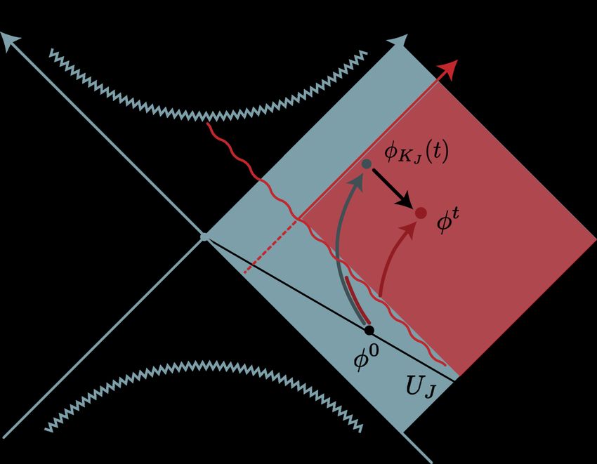
Contents

1 Inside a quantum system                                                                               1
2 Boundary description of bulk observers                                                                3
  2.1 A black hole “observer”                                                                           4
  2.2 Tracing out the observer: modular Hamiltonian and Berry transport                                 6
  2.3 The observer’s code subspace                                                                      8

                                                                                                             JHEP03(2022)084
3 The      holographic measurement of time                                                            10
  3.1      The proposal: proper time from modular time                                                10
  3.2      A test case: moving black holes in AdS                                                     15
  3.3      Time dilation for twin observers                                                           17
4 Particle detection                                                                                  18
  4.1 Modular flow in the presence of infalling matter                                                19
  4.2 Energy distribution from maximal modular chaos                                                  24
5 Discussion                                                                                          26
  5.1 Resolution of the Marolf-Wall puzzle                                                            26
  5.2 The frozen vacuum problem                                                                       28
  5.3 How small can our probe black hole be?                                                          28
  5.4 Emergent time                                                                                   31

1       Inside a quantum system

Suppose your adventurous colleague jumped in the AdS black hole you created in your lab’s
quantum computer by simulating N = 4 Super Yang-Mills. What did their Geiger counter
register along their journey and at what age did they meet their inevitable end?
     Gauge/gravity duality [1] has offered a wealth of insights on the microscopic description
of black holes, as observed from an asymptotic frame. These include their entropy, fast
scrambling dynamics [2, 3] and unitarity of the Hawking evaporation process [4, 5]. In
contrast, the infalling observer’s experience remains mysterious, owing to the lack of
holographic reconstruction techniques that penetrate bulk horizons. The difficulty in posing,
even in principle, operationally meaningful questions such as the amount of time or energy
measured by observers behind horizons highlights a gap in our understanding of AdS/CFT:
the absence of a CFT framework for describing physics in an internal reference frame.
     To catalyze progress in this direction, we pursue an observer-centric approach to bulk
reconstruction.1 Even for observers that do not fall into black holes, no general method for
    1
    Related attempts to describe physics from an internal observer’s point of view include [6, 7], as well
as the series of works [8–11] which includes a few interpretational claims that deviate somewhat from the
proposal presented in this paper.

                                                  –1–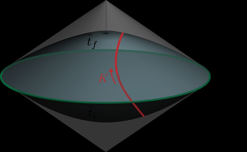
determining how their experience is encoded in the CFT is known, particularly without
having to solve the bulk theory directly. This is closely related to the fact that CFT
operators are attuned to an external description of the quantum system, while the observer
is associated to an internal frame of reference.
     Any observer made out of bulk matter is simply a suitable subsystem of the dual
Conformal Field Theory.2 In our work, this observer will be a black hole entangled with an
external reference; the subsystem available for their experiments consists of operators within
the black hole “atmosphere” (section 2). The entangled reference provides an external way
to describe the frame associated to the observer. The virtue of such a probe black hole is in
providing a particularly simple model of a subsystem, related by a unitary transformation

                                                                                                           JHEP03(2022)084
to the thermofield double state [12].
     The probe black hole will be introduced near the boundary, and then allowed to
propagate under time evolution before returning to our possession at a later time. 3 The
only assumption about the bulk state we make is that it is described by a semi-classical
spacetime, whose features we wish to probe in the classical limit. In this setup, we start
by solving the following problem: assuming CFT knowledge of the atmosphere degrees
of freedom at the initial and final timeslices, and of the CFT Hamiltonian, how much
proper time did the observer’s clock measure and what energy distribution was detected by
their calorimeter?
     In sections 3 and 4, we explain how to read off this information from the boundary
unitary VH (0, t) that relates the initial (ti = 0) and final (tf = t) local atmosphere operators.
The result is universal within its domain of validity, and does not require as an input
the solution for the bulk spacetime. The key ingredient is the modular Hamiltonian of
the black hole, K = − log ρ, defined by its reduced density matrix ρ after tracing out the
reference system. In a nutshell, we propose that the decomposition of log VH in terms of
(approximate) “eigen-operators” of K has the schematic form:

                      τ (t)                      τ (t)
                              Z
  i log VH (0, t) =               dΩd−2 f (Ω) G2π (Ω) +K + other zero-modes + O(e−τ , N −1 )
                       2π                         2π
                                                                                          (1.1)
The coefficient τ (t) of the modular operator is the proper time. G2π (Ω) are the modular
scrambling modes, satisfying [K, G2π ] = −2πiG2π [13] thus growing exponentially under
modular flow, and the coefficient f (Ω) depends on the expectation value of the horizon
null energy flux x+ =0 dx− hT−− i in the frame of the moving black hole. A non-vanishing
                 R

scrambling mode coefficient in (1.1) is, therefore, a signature of particle detection along the
bulk worldline. The other zero mode contributions describe the precession of the observer’s
symmetry frame, e.g. a local rotation about the black hole. Our result is valid when the
proper time is shorter than the scrambling time of our probe black hole τ (t) . log SBH .
     The basic intuition, from the point of view of the quantum system, is that proper
time is measured by the phase, eimτ , of the state, as in Feynman’s path integral for a
   2
     Our construction does not rely on conformal symmetry. This generality is crucial for it to apply in
non-vacuum states with semi-classical bulk duals.
   3
     This precludes exploring behind horizons in the particular setup of this work. Nevertheless, our
framework contains lessons for black hole interior reconstruction which we discuss in section 5.

                                                   –2–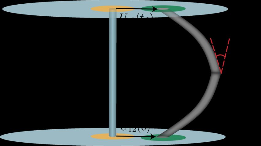
particle worldline. In our setup, the analog of the rest mass, m is provided by the local
energy, conveniently given by the Hamiltonian of the reference system which is exactly
AdS Schwarzschild. This corresponds to the modular Hamiltonian for the spacetime being
probed. An important additional ingredient is that we keep track of the unitary VH (0, t)
that relates the presumed known operator algebra of the probe black hole atmosphere at the
beginning and end of its journey through the bulk, to correctly translate between the initial
and final states. This is necessary to have a well-defined comparison without requiring
the input of a collection of CFT operators associated to translations in a particular bulk
time slicing.
     In the bulk language, we use the fact that the modular Hamiltonian acts approximately

                                                                                                 JHEP03(2022)084
as the local Schwarzschild time evolution relative to the extremal surface, in a sense that
we make more precise below. An important point is that because the total state is a single
sided unitary transformation of the thermofield double, the corrections to the geometric
action of the modular flow can be regarded as transients due to excitations of the bulk fields
near the probe black hole, which in our setup do not affect the initial and final atmosphere
operators. The only persistent effect is a shift of the extremal surface relative to the probe
black hole causal horizon, with respect to which we wish to define the atmosphere operators.
This is encoded by the scrambling modes in eq. (1.1) and is explained in detail in section 4.
     In section 3.3, we employ this technology to holographically measure the time dilation
witnessed by two twins who embark on separate journeys and compare clocks at their future
reunion. In the dual quantum description, the twins select two time-dependent families
of modular Hamiltonians, describing the evolution of their state, which are simply related
when the siblings meet at the initial and final moments, thus forming a “closed loop”. The
proper time difference experienced by the twins is computed by two intrinsic properties of
this modular loop: the modular Berry holonomy [14–16] (section 2.2) and the modular zero
mode component of the CFT Hamiltonian integrated along the path.
     The experience of an observer falling into a black hole is discussed in section 5. Our
framework naturally resolves a conceptual puzzle raised by Marolf and Wall [17] regarding
the ability of an observer that enters from one side of an AdS wormhole to receive signals
coming from the other, despite the dynamical decoupling of the two exterior regions.
Moreover, our proposal outlines an interesting perspective on the “problem of time” in
quantum gravity in general, an early form of which was anticipated in [18]. Our eq. (1.1)
links the geometric notion of time in General Relativity to the natural, quantum mechanical
clock of the dual theory, the modular clock, obtained by tracing out the “observer”. It,
thus, seems to enjoy a degree of universality that may extend its validity beyond the
AdS/CFT context.

2   Boundary description of bulk observers

In this paper, we model a bulk observer as a black hole. It will be a large black hole, in the
sense of having a Schwarzschild radius of order the AdS curvature scale, as required for
having a simple associated modular flow. However, we will take it to be much smaller than

                                            –3–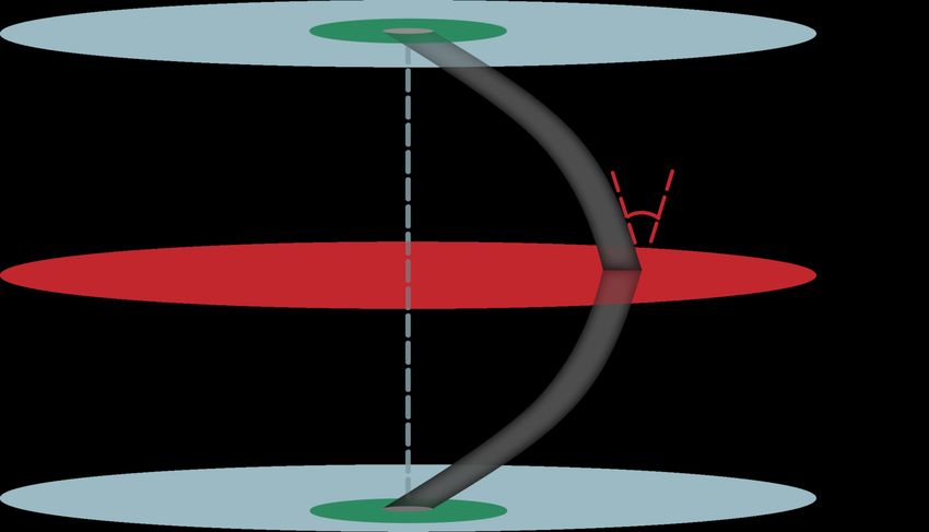
the features of the spacetime that it is intended to probe. For this reason our construction
captures AdS scale locality and geometric features.
     It is, of course, very interesting to generalize the approach to small black holes, whose
associated modular flows are less universal. The microcanonical eternal black holes of [19]
are the natural candidate for such a generalization, since they are semiclassical configurations
black holes whose horizon radius can be parametrically smaller than LAdS while being
thermodynamically dominant within an energy window. We discuss this generalization and
related subtleties in some detail in section 5.
     This section summarizes the advantages of the probe black hole description and
introduces the concepts we will utilize in articulating our proposal in sections 3 and 4: the

                                                                                                   JHEP03(2022)084
modular Hamiltonian, modular Berry transport and the observer’s code subspace degrees
of freedom.

2.1   A black hole “observer”
The textbook observer in General Relativity is a local probe: they have zero size, no gravi-
tational field and they travel along a worldline whose local neighborhood is approximately
flat. This is a convenient idealization in the classical theory which, however, is unavailable
quantum mechanically. Quantum observers are physical systems that should be included
in the wavefunction of the Universe. They have finite mass and occupy volume of some
linear size ` necessarily larger than their own Schwarzschild radius but smaller than the
curvature scale of the spacetime they live in. Their gravitational field changes the local
geometry around them to approximately Schwarzschild in their local inertial frame and
quantum mechanical evolution entangles them with their environment —a potential deco-
herence they need to protect themselves against to stay alive. Last but not least, observers
have agency: they can manipulate and measure degrees of freedom in their vicinity to
perform experiments.
     A general treatment of internal observers in AdS/CFT is a hopeless task but, fortunately,
an unnecessary one. All we need is a more appropriate idealization of the physical observer
above. In this paper, we squeeze our observer down to their Schwarzschild radius, collapsing
them to a black hole of size rBH which we thermally entangle with an external reference
system (figure 1). This black hole “observer” will approximately propagate along the same
worldline, leaving the physics at scales much larger than rBH unaffected. The only difference
is that excitations that originally intercepted the worldline are now absorbed by our black
hole: they get detected by our observer’s device!
     The entangled external system provides a precise meaning to the reference frame of
the observer. In particular, one could consider gravitational operators probing the system
spacetime whose diffeomorphism dressing is attached to the reference boundary through the
Einstein-Rosen bridge. These must be complicated operators acting on both system and
reference quantum systems, whose action in a (non-factorized) code subspace approximates
that bulk description.
     In this work, we will be able to phrase our final results without needing such operators,
which agrees with the fact that the proper time along the probe’s trajectory between known
near-boundary initial and final configurations is diffeomorphism invariant without requiring

                                             –4–
JHEP03(2022)084
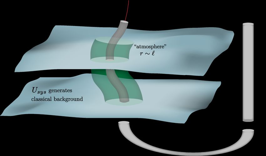
Figure 1. An illustration of our setup. The red line represents the worldline of an ideal observer.
We replace them by a small black hole of radius rBH much smaller than the spacetime’s curvature
features which we thermally entangle with a reference system, assumed to be another AdS black hole
for simplicity. The black hole propagates along the original geodesic due to the equivalence principle.
The green tube of radius ` around the black hole represents its “atmosphere”: the operators our
observer can manipulate at any given time.
the observer’s frame. As such, only system framed atmosphere operators and the probe
black hole’s density matrix appear in formula for the proper time. However, it is interesting
to compare the result to the clock of the reference system, which gives a simple way to
understand our results.
Assuming the reference is a copy of the original CFT for simplicity, and that rBH ∼
LAdS , the initial global state describing a black hole inserted somewhere in a classical,
asymptotically AdS background has the general form:
|Ψi = Z −1/2 e−βEn /2 Usys |En isys |En iref (2.1)
X
n
where Usys is a unitary transformation that excites the bulk fields and metric to create the
background our black hole will propagate in.4 Note that any state which looks like the
eternal black hole in the reference system must be of this form.
Crucially, collapsing our observer to a black hole offers protection from decoherence:
its degrees of freedom will remain spatially localized in the bulk for a time-scale of order
4
Black holes with rBH
LAdS could also in principle be discussed in our formalism, with the difference
that the system-reference state would be more complicated since small black holes do not dominate the
canonical ensemble. See section 5 for related discussion.
–5–the evaporation time which we will assume to be much larger than the time-scales of the
experiments we will perform.
We choose a black hole “atmosphere” of size ` to be the observer’s lab: local operators
in the atmosphere can be directly manipulated or measured. We will assume rBH . LAdS
`
L where L the scale of the spacetime curvature perturbations about AdS. The CFT
duals of the atmosphere operators at different times select a time-dependent subsystem of
the boundary theory. This family of (abstract) CFT subsystems serves as a quantum notion
of our observer’s local frame which will be important in our formalism and is explained
further in section 2.3.
JHEP03(2022)084
2.2 Tracing out the observer: modular Hamiltonian and Berry transport
An observer’s description of the Universe they inhabit does not include a description
of themselves. The degrees of freedom that make up the observer, which are generally
entangled with the rest of the bulk, ought to be traced out. For the idealized eternal black
hole observer of section 2.1 this corresponds to tracing out the reference system.
Modular Hamiltonian. Entanglement leads to uncertainty about a subsystem’s quan-
tum state. In our setup, ignorance of the state of the reference results in a mixed state
ρ = Trref [|ΨihΨ|] for our black hole system. The Hermitian operator K = − log ρ is the
modular Hamiltonian and it defines an automorphism of the operator algebra. The action
of this automorphism is generally non-local, except in special situations, and it can be
thought of as generating the “time” evolution with respect to which the subsystem is in
equilibrium. Somewhat more formally [20], the modular Hamiltonian of a quantum field
theory subsystem in the state Ψ is defined as K = − log ∆Ψ where ∆Ψ is the “KMS operator”
of Ψ satisfying:
hΨ|φ†1 ∆Ψ φ2 |Ψi = hΨ|φ2 φ†1 |Ψi (2.2)
for all correlation functions of the subsystems’s operator algebra.
For our class of states (2.1), the modular Hamiltonian is unitarily equivalent to the
dynamical Hamiltonian of the boundary theory:
†
K = 2π Usys HUsys (2.3)
β
where we have renormalized H to 2π H, for convenience. Recall that this is actually the most
general type of state in which the full spacetime is identical to empty AdS-Schwarzschild
on the reference side. In Schrodinger picture, time evolution acts on the state, resulting in
a time-dependent modular Hamiltonian K(t).
A simple example we will frequently use to illustrate the ideas of this paper is a boosted
black hole, which bounces back and forth in AdS. This is prepared by acting on a static black
hole with the asymptotic boost symmetry of the spacetime, generated by the conformal
boost B in the CFT. Its dual state corresponds to (2.1) with the choice Usys = e−iBη , where
η the black hole’s rapidity, and the time dependent modular Hamiltonian reads explicitly:
(2π)−1 K(t) = cosh η H + sinh η(P cos t + B sin t) (2.4)
–6–where H, P, B the conformal generators satisfying the usual SL(2, R) algebra:
[B, H] = iP , [B, P ] = iH , [H, P ] = iB (2.5)
Modular Berry Wilson lines. A continuous family of modular Hamiltonians K(t)
—like eq. (2.4)— selects a continuous family of bases in the Hilbert space, consisting of
the eigenvectors of K(t). The local generator D(t) of the basis rotation can generally be
obtained as the solution to the problem:
∂t K(t) = −i[D(t), K(t)] (2.6)
JHEP03(2022)084
Equation (2.6) by itself determines D(t) only up to modular zero modes Q(t), generating
symmetries of the reduced state [Q(t), K(t)] = 0. This reflects the freedom to choose at will
the local modular frame, e.g. phases of eigenstates of different K(t), which is an example
of a Berry phase, discussed in detail in [16]. A canonical map between the bases that is
intrinsic to the family K(t) can be constructed following Berry’s footsteps [21], by defining
the modular parallel transport operator as the solution to the problem (2.6) supplemented
by the condition:
P0t [D(t)] = 0 (2.7)
where P0t is the projection of the Hermitian operator D(t) onto the subspace of zero modes
of K(t). Eigenframes of different K(t) are related by modular Wilson lines, the path ordered
exponential of the parallel transport D(t)
Z t2
0 0
W(t1 , t2 ) = T exp −i dt D(t ) (2.8)
t1
W can also be thought of as a canonical unitary automorphism of the operator algebra of
our system:
OW (t) = W(0, t) O W † (0, t) (2.9)
with the properties:
K(t) = W(0, t) K(0) W † (0, t) (2.10)
(1) (n)
hΨ(t)| OW (t) . . . OW (t) |Ψ(t)i = hΨ| O(1) . . . O (n) |Ψi (2.11)
When K(t) is obtained via the time evolution of the system —as in the example
of the previous subsection— the modular parallel transport is related to the, possibly
time-dependent, Hamiltonian H(t) via:
D(t) = H(t) − P0t [H(t)] (2.12)
In our boosted black hole example with modular Hamiltonian (2.4), the parallel transport
problem can be solved explicitly by a straightforward group theory exercise. A convenient
–7–way to express the solution is:
D(t) = ẋ(t) P + η̇(t)e−iP x(t) B eiP x(t) − b(t) K(t) (2.13)
x(t) = tanh−1 (tanh η(0) sin t) (2.14)
−1
η(t) = sinh (sinh η(0) cos t) (2.15)
1
b(t) = ẋ(t) sinh η(t) (2.16)
2π
where x(t), η(t) measure the black hole’s geodesic distance from the AdS origin and its
rapidity in the global frame respectively, while the last term enforces the vanishing of the
JHEP03(2022)084
zero-mode component of D(t). The modular parallel transport operator (2.8) then reads:
Z t Rt
i
dt0 ẋ sinh η(t0 )
Wboosted BH (0, t) = T exp −i dt0 D(t0 ) = e−iP x(t) e−iB(η(t)−η(0)) e 2π K(0) 0
0
(2.17)
Modular holonomies. A key property of the modular Berry transport is that it generally
leads to non-trivial holonomies —a fact that will play an important role in our subsequent
discussion. We can consider two families of modular Hamiltonians, K1 (t), K2 (t) for t ∈ [0, T ],
which coincide at the initial and final times: K1 (0) = K2 (0) and K1 (T ) = K2 (T ). These
could correspond to two distinct worldlines for our black hole that begin and end at the same
spacetime location and with the same momentum. K1 (t), K2 (t) then form a closed “loop”
K (t) 0≤t≤T
1
K(t) = (2.18)
K (2T − t), T ≤ t ≤ 2T
2
and the property (2.10) becomes:
†
K(0) = Wloop (0, 2T ) K(0) Wloop (0, 2T ) (2.19)
which implies that the modular Wilson loop, Wloop (0, T ) will be a, generally non-trivial,
element of the modular symmetry group, generated by the zero modes Qi (0):
" #
Wloop (0, T ) = exp −i di Qi (0) (2.20)
X
i
This is a modular Berry holonomy, an example of which we will see below in our discussion
of time dilation between observers.
2.3 The observer’s code subspace
Up to this point, we have treated the bulk observer as a physical system, entangled with
their environment in the global wavefunction, which results in a time-dependent modular
Hamiltonian K(t) upon tracing them out. Another defining characteristic of an observer,
however, is their ability to control some degrees of freedom in their Universe to learn about
Its state. In our model, these will be the local bulk fields in a small atmosphere of size `
around the black hole, denoted by φi with i an abstract index, and O(1)−degree polynomials
built out of them and their derivatives.
–8–The atmosphere degrees of freedom on a particular bulk timeslice Σt which asymptotes
to boundary time t form a set of observables
St ≡ {φi (xi ), φj (xj )φl (xl ), ∂φk (xk ), . . . xi ∈ Σt and |xi − xH | ≤ `} (2.21)
By acting with elements of St on the background state (2.1) we obtain the observer’s
instantaneous code subspace [22]: the subspace of the CFT Hilbert space the observer can
explore with their apparatus at a given bulk time. Crucially, this code subspace is not
generally preserved by time evolution. The observer moves in the bulk hence the operators
in their vicinity (and their boundary duals) differ at different times, resulting in an evolution
JHEP03(2022)084
of the CFT subspace that the observer can probe.
As remarked in our introductory section, we will assume knowledge of the CFT duals
of the atmosphere operators at an initial and a final timeslice, Sti and Stf respectively
—but not in-between. This is physically reasonable when studying processes where the black
hole is introduced far out in the asymptotically AdS region and returns to it at some later
boundary time, in which case the familiar HKLL prescription for an AdS black hole can be
employed for the initial and final reconstruction.
Dressing. Sti , Stf refer to local operators in a theory of gravity so it is important to
clarify their gravitational framing. The choice of an initial and final timeslices Σti , Σtf in
the definition of the operator sets is a selection of a bulk gauge, at least in the vicinity
of the black hole. Since the black hole is assumed to be near the AdS boundary at those
moments, its local neighborhood is diffeomorphic to an AdS-Schwarzschild geometry. These
local AdS-Schwarzschild coordinates serve as the analog of the local inertial frame about an
idealized observer’s worldline. We are interested in describing the operators in the black
hole’s reference frame, thus we choose Σti , Σtf to both be constant time with respect to the
corresponding local time-like killing vector within the atmosphere (figure 2). Operators
φ ∈ Sti or Stf can then be labelled by their location in this local AdS-Schwarzschild
coordinate system.
These are operators that are dressed with respect to the AdS boundary with the
property that their action within the code subspace results in their insertion at given
positions relative to the “local horizon”, namely the place where the horizon would form if
no matter were absorbed in the future. This “local horizon” may generally differ for Sti and
Stf , as we will see in section 4. Using standard HKLL, we can construct such operators
that work in an entire family of perturbative excitations about a black hole of a given
temperature [23, 24].
It is important to note that when acting within the code subspace of small perturbations 5
around a given semi-classical spacetime state, bulk operators with different dressings that
result in insertion at the same point in the original spacetime are equal at leading order.
The associated states φ|Ψi would appear to have different gravitational field configurations
associated to the energy of the particle produced by φ, however these are subleading to
the quantum fluctuations in the ambient gravitational field. This can be seen by explicitly
5
The perturbations must be small at the specified time, to avoid exciting scrambling modes that lead to
large deviations —as we explain in section 4.
–9–computing the overlap of two such states with different dressings for φ that classically result
in the same insertion point. The states are identical as quantum states up to GN corrections.
Example. For illustration, we return to our boosted black hole example (2.4). The
atmosphere operators at the t = 0 global AdS timeslice, when the black hole is located at
the AdS origin and has rapidity η, can be obtained from the standard HKLL operators in a
static AdS-Schwarzschild metric via the action of a boundary conformal boost:
φ0 (r, Ω) = e−iBη φstatic (r, Ω) eiBη where: `P l
r − rBH < ` (2.22)
After global time t the black hole has moved to a new location x(t) and has a local rapidity
JHEP03(2022)084
η(t) given in (2.14) and (2.15). By the previous reasoning, the atmosphere observables, in
the Schrodinger picture, are given by:
φt (r, Ω) = e−iP x(t) e−iBη(t) φstatic (r, Ω) eiBη(t) eiP x(t) where: `P l
r − rBH < ` (2.23)
Proper time evolution. The unitary that relate the atmosphere operators St at different
times t is, by definition, the proper time evolution along the black hole’s worldline. We
will denote this unitary by VS (t1 , t2 ) or VH (t1 , t2 ) depending on whether we represent it
in the Schrodinger or Heisenberg picture. The goal of the remainder of this paper is to
understand the construction of V directly in the CFT language, without reference to bulk
reconstruction —except at the initial and final moments of our probe black hole’s history.
3 The holographic measurement of time
With all the necessary concepts in place, we are ready to present the advertised connection
between modular time and proper time, when no matter gets absorbed by our probe black
hole; the case of particle absorption is postponed for section 4.
3.1 The proposal: proper time from modular time
We now provide three complementary perspectives on our main claim. We start with a
bulk geometric argument that offers some useful intuition and then make the case quantum
mechanically, using both Heisenberg and Schrodinger picture reasoning, each of which
illuminates different aspects of the physics.
An intuitive geometric argument. In the bulk, our black hole observer can be under-
stood via the geometric construction of figure 2. We start with an idealized probe observer
of some small mass m and we choose an initial Cauchy slice Σ0 which is “constant time” in
their local inertial frame, as well as the Cauchy slices within an → 0 thickness time band
Σ0 () around it. The geometry of this time band near the observer’s location reads, in local
inertial coordinates:
r
µ µ
ds2obs ≈ −dτ 2 + dr2 + r2 dΩ + d−3
(dτ 2 + dr2 ) + O (Lx)2 (3.1)
r
where τ is the proper length of the worldline, r the radial distance from it and L is the
scale of the curvature features of the surrounding spacetime.
– 10 –JHEP03(2022)084
Figure 2. Our black hole is introduced geometrically by cutting a hole of size ` around the ideal
observer’s worldline in the initial Cauchy slice and a small time band Σ0 () about it and replacing
the interior with a black hole metric. The local killing vector generating the worldline’s proper time
is glued to the local generator of Schwarzschild time which, in turn, is modular time. As long as
nothing falls in the black hole, this identification is valid everywhere along the worldline, suggesting
that modular time is correlated to proper time.
1
We cut a hole of size ` in Σ0 (), with µ d−3
`
L, around the worldline and replace
its interior with the black hole geometry:6
−1
µ µ
rHamiltonian [25, 26] which, in turn, is defined via the KMS operator (2.2)
hΨ|φ†1 e−K φ2 |Ψi = hΨ|φ2 φ†1 |Ψi (3.3)
As long as particles do not cross paths with our black hole’s trajectory, the state of the
black hole atmosphere will remain in an approximate local thermal equilibrium: expectation
values of atmosphere observables will be approximately given by their thermal ones, with
the Wick rotation of the local timelike killing direction ts playing the role of the thermal
circle. By virtue of the usual KMS condition then, we have
JHEP03(2022)084
hΨ|φ†1 e−K φ2 |Ψi = hΨ|φ2 φ†1 |Ψi ≈ hΨ|φ†1 e−2πPξs φ2 |Ψi (3.4)
where: Pξs the geometric generator of the geometric flow of ξs . Hence, within the local
thermal atmosphere r . `, K acts like the geometric generator 2πPξs which coincides with
the worldline proper time generator 2πPξτ at r ∼ `.
Heisenberg picture. To justify our proposal quantum mechanically, it is simplest to
work in the Heisenberg picture. Hamiltonian evolution of the system is described by
the unitary rotation of the operator basis, while the state and by extension the modular
Hamiltonian remain fixed. The atmosphere operator set St of section 2.3, however, does
not simply consist of the Heisenberg evolved elements of S0 , because their correct evolution,
which we denote by the unitary VH (0, t), needs to also reflect the motion of the black hole
in the gravity dual:
φtH (x) = VH (0, t) φ0H (x) VH† (0, t) (3.5)
where the subscript H is introduced to make the Heisenberg picture explicit. Given our
assumption that
1. the black hole on the initial and final timeslices Σ0 , Σt is located in the asymptotic
AdS region and is thus locally diffeomorphic to AdS-Schwarzschild, with the state
being approximately invariant under the local killing time-like vector
2. no energy is absorbed by our probe black hole —an assumption we lift in section 4
we conclude that correlation functions of Heisenberg operators in S0 and St are identical in
the background state |Ψi:
hΨ| φtH,1 . . . φtH,n |Ψi = hΨ| φ0H,1 . . . φ0H,n |Ψi (3.6)
The meaning of these operators are bulk fields, dressed to the AdS boundary in such a
way that in the subspace under consideration they are inserted in the atmosphere as labeled
by coordinates relative to the extremal surface. Due to the Schwarzschild time-like isometry
of the near horizon region, one needs to additionally specify a timeslice, anchored to the
AdS boundary. We can do this because we assume that the black hole begins and ends its
journey in understood regions near the boundary.
– 12 –Due to (3.6), the isomorphism VH (0, t) must be a “modular symmetry”, when acting on
the observer’s code subspace. Such a unitary can be generated by two classes of operators:
• zero modes Qa of the modular Hamiltonian projected onto the observer’s code subspace:
[Qa , Pcode K(0)Pcode ] = 0, where: Hcode = {O|Ψi, ∀ O ∈ S0 } (3.7)
• operators Gλ = G†λ that are eigenoperators of the code subspace K with imaginary
eigenvalues
[Pcode K(0)Pcode , Gλ ] = −iλGλ (3.8)
JHEP03(2022)084
The latter necessarily annihilate state |Ψi since otherwise Gλ |Ψi would constitute an
eigenstate of the modular Hamiltonian with imaginary eigenvalue which contradicts the
Hermiticity of K. A special class of these imaginary eigenvalue operators is those with
λ = ±2π. These were dubbed modular scrambling modes in [13] because they saturate
the bound on modular chaos and they were argued to generate null translations near the
entangling surface. The simplest example of such a scrambling mode is the Averaged Null
Energy operator dx+ T++ (Ω) at the horizon of a static AdS black hole in equilibrium,
R
where the eigenvalue 2πi follows from the near horizon Poincare algebra.
We claim that Gλ do not contribute to the unitary VH when no particles get absorbed
by our black hole. This is not true for cases with non-vanishing infalling energy flux which,
as we show in section 4.1, results in a scrambling mode G2π contribution. Modes with
|λ| > 2π are forbidden by the modular chaos bound [13, 27], as we review in section 4.2.
We are unaware of any situations where Gλ with −2π < λ < 2π appear, thus we tentatively
suggest they are, also, absent in general —leaving a more thorough investigation of this
issue for future work. With some foresight, we can return to the case with no absorption
and express the evolution operator in (3.5) as:
τ (t)
" #
VH (0, t) = exp −i da (t)Q0a (3.9)
X
K(0) − i
2π a
where we separated the modular Hamiltonian from the rest of the zero modes Q0a . We
propose that the coefficient of the modular Hamiltonian τ (t) measures the proper time along
the bulk observer’s worldline, in units of the black hole temperature β/2π. The other zero
modes Q0a describe the precession of the symmetry frame of the observer, e.g. a certain
amount of rotation of the local reference frame.
The intuition for identifying τ (t) with proper time is as follows. Within the code
subspace, the action of the atmosphere φ is, at leading order, identical to bulk operators
that are framed to the reference boundary, at an appropriate time. Evolution under the
reference Hamiltonian moves the anchor point of those operators, and this gives the local
Schwarzschild evolution in the atmosphere region. Thus the proper time along the trajectory
is exactly the amount of modular evolution required to relate the initial and final atmosphere
operators, where we equate operators with equal projection onto the code subspace.
– 13 –JHEP03(2022)084
Figure 3. Illustration of the three different flows appearing in our discussion. H is the CFT
Hamiltonian generating global AdS evolution. VH is modular flow which maps the ti = 0 atmosphere
operators (green disk on ti = 0 slice) to the Heisenberg picture atmosphere operators at tf = t. VS
describes the evolution of the atmosphere operators in the Schrodinger picture and captures the
motion of the black hole relative to the boundary.
Schrodinger picture. It is illuminating to present the same argument in the Schrodinger
picture, where the black hole state in what evolves under the Hamiltonian evolution, as
encapsulated in a time-dependent K(t). While, now, the operator basis does not evolve,
the atmosphere operator set St does, due to the motion of the bulk black hole relative to
the AdS boundary. The Schrodinger picture atmosphere operators in S0 and St are related
by a unitary VS (0, t):
φt (x) = VS (0, t) φ0 (x) VS† (0, t) (3.10)
where the subscript S is a reminder that we are working in the Schrodinger picture.
The Schrodinger version of eq. (3.6) is that correlation functions of operators in S0 in
the initial state |Ψi are equal to correlation functions of the final atmosphere operators St
in |Ψ(t)i:
hΨ(t)| φt1 . . . φtn |Ψ(t)i = hΨ| φ01 . . . φ0n |Ψi (3.11)
By virtue of eq. (2.11), property (3.11) the isomorphism (3.10) can be identified with
the modular Berry transport W, up to a symmetry ZQ of the observer’s code subspace
correlators:
VS (0, t) = W(0, t) ZQ [ca (t)] (3.12)
" #
where: ZQ [ca (t)] = exp −i ca (t)Qa (0) (3.13)
X
a
and, as before, Qa are the code subspace modular zero-modes (3.7).
– 14 –As explained in section 2.2, for a family K(t) obtained by Hamiltonian time evolution
W is generated by (2.12) so (3.12) becomes:
Z t
0 0
VS (0, t) = T exp −i dt (H − P0t [H]) ZQ [ca (t)]
0
h Z t 0 0 0
i
= e−iHt exp i dt0 eiHt P0t [H]e−iHt ZQ [ca (t)] (3.14)
0
Substituting (3.14) in eq. (3.10) and switching to the Heisenberg picture we get the following
relation between the atmosphere operators:
φtH (x) = VH (0, t) φ0H (x) VH† (0, t)
JHEP03(2022)084
h Z t 0 0 0
i
where: VH (0, t) = exp i dt0 eiHt P0t [H]e−iHt ZQ [ca (t)] (3.15)
0
The unitary VH is now obtained by the product of two contributions, one coming from the
zero-mode projection of the CFT Hamiltonian and the other from the code subspace sym-
metry transformation ZQ in (3.12). These two terms have distinct physical interpretations
which we discuss in the context of our AdS example below. This decomposition will be
important in our discussion of the relative time between two observers in section 3.3, where
the ZQ contributions will give rise to a modular Berry holonomy, providing a conceptually
clean way of organizing the CFT dual of time dilation.
3.2 A test case: moving black holes in AdS
As an illustration of the idea, we focus on black holes moving in empty AdS along arbitrary
worldlines and compute their proper time using our proposed method.
AdS black holes in inertial motion. Consider the case of the boosted black hole,
propagating along an AdS geodesic. In the CFT, it is characterized in the Schrodinger
picture by the time-dependent modular Hamiltonian (2.4), with atmosphere operators on
the initial and final timeslices given by (2.22) and (2.23) respectively. The unitary VS (0, t)
in eq. (3.10) is equal to:
VS (0, t) = e−iP x(t) e−iB(η(t)−η(0)) (3.16)
Recalling the expression (2.17) for the modular parallel transport in this example, VS can
be written as:
Z t
−1 0 0 0
VS (0, t) = Wboosted BH (0, t) exp −i(2π) K(0) dt ẋ(t ) sinh η(t ) (3.17)
0
Equally straightforwardly, we can compute the projection of the dynamical Hamiltonian on
the modular zero modes of K(t), which reads:
1
P0t [H] = cosh η(0)K(t) (3.18)
2π
Combining the results (3.17) and (3.18) in expression (3.15) for the proper time evolution
operator VH (0, t) we find:
Z t
−1 0 0 0
VH (0, t) = exp −i(2π) ẋ(t ) sinh η(t ) − cosh η(0) (3.19)
K(0) dt
0
– 15 –The coefficient of the modular Hamiltonian, using the expressions (2.14) and (2.15) for x(t)
and η(t), reads:
tan t
τ (t) = tan−1 (3.20)
cosh η(0)
which is indeed the proper length of the black hole’s worldline between the 0 and t global
AdS timeslices.
A worldline interpretation of the result. At a sufficiently coarse-grained level, our
black hole behaves like a particle, whose propagation in the bulk spacetime follows from
extremization of its worldline action, i.e. its proper length
JHEP03(2022)084
Z Z t
Sworldline [xµ (t)] = dτ = dt0 L(xµ (t), ẋµ (t)|g) (3.21)
0
which can alternatively be written as a Legendre transform of the worldline energy E[xµ (t)]:
Z t
δL
Sworldline [xµ (t)] = dt ẋµ − E[xµ (t)] (3.22)
0 δ ẋµ
It is instructive to observe that the two zero mode contributions to VH in eq. (3.15) have
different physical interpretations. The zero mode of the CFT Hamiltonian (3.18) measures
the energy of the black hole E[xµ (t)], namely the worldline Hamiltonian evaluated on-shell,
while the zero mode contribution to (3.17) in the chosen gauge is equal to the quantity
ẋµ (t) δδL
ẋµ along the trajectory. The two are combined in eq. (3.19) to give an amount of
modular evolution equal to the on-shell worldline action for our probe black hole.
Accelerating AdS black holes. The example can be extended to arbitrary accelerating
black holes. A simple example is a black hole that starts at the AdS origin at t = 0 with
rapidity η(0) and at some boundary time t0 receives a kick that changes its rapidity, e.g.
flips it from η(t0 ) to −η(t0 ). The black hole returns to the origin at global time t = 2t0 when
its internal clock is showing τ (2t0 ) = 2 tan−1 cosh η(0) , according to the bulk calculation.
tan t0
The modular Wilson line associated to the corresponding family of modular Hamiltoni-
ans can be computed straightforwardly from its defining equations (2.6), (2.7):
R 2t0
dt0 D(t0 )
W(0, 2t0 ) = T e−i 0
h i
= Wboosted BH (π − t0 , π) exp 2iBx(t0 ) η(t0 ) Wboosted BH (0, t0 ) (3.23)
where Wboosted BH is given by (2.17), and the instantaneous boost Bx(t0 ) = e−iP x(t0 ) B eiP x(t0 )
accounts for the t = t0 discontinuity in the operator family K(t) due to the kick of the
black hole. This discontinuity is, of course, an artifact of our approximation that would be
absent from any realistic accelerating black hole.
On the boundary, the local atmosphere fields at t = 0 and t = 2t0 are related by
φ2t0 = e2iBη(0) φ0 e−2iBη(0) (3.24)
In view of (3.23), the map VS (0, 2t0 ) = e2iBη(0) in (3.24) can be shown to be equal to
Z t0
−1 0 0 0
VS (0, 2t0 ) = W(0, 2t0 ) exp −2i(2π) K(0) dt ẋ(t ) sinh η(t ) (3.25)
0
– 16 –Figure 4. LEFT: a black hole in AdS that receives a kick at t0 . Arbitrary trajectories in AdS
JHEP03(2022)084
can be generated by a dense sequence of such instantaneous kicks, allowing us to describe proper
time evolution in any weakly curved spacetime. RIGHT: twin black holes. The left twin is static
while the right twin is the accelerated black hole of the LEFT panel. The time dilation experienced
by the twins is computed by the modular Berry holonomy of the “loop” of modular Hamiltonians
describing the two trajectories and the integral of the zero mode projection of the CFT Hamiltonian
along the loop via eq. (3.28), (3.29).
Extracting the proper time requires computing the Heisenberg picture evolution opera-
tor (3.15). The zero mode component of the CFT Hamiltonian is once again given by (3.18)
so the final result reads
tan t0 K(0)
−1
VH (0, 2t0 ) = exp −2i tan (3.26)
cosh η(0) 2π
which agrees with the bulk geometric computation.
By an appropriate dense sequence of small kicks like the one studied here, an arbitrary
worldline can be constructed, allowing our method to correctly compute the proper length
of any timelike path in AdS. This construction guarantees that our prescription works in
all weak curvature perturbations of Anti-de Sitter spacetime.
3.3 Time dilation for twin observers
The proper time measured by a bulk observer is a gauge dependent quantity, being a
function of the initial and final points between which the proper length of the worldline
is computed. This fact was reflected in our previous discussion in the choice of the bulk
slices Σti and Σtf on which the atmosphere operators are defined. Waiving the need for the
latter requires asking a gauge invariant question.
In this section, we are interested in computing the relative time, or time dilation,
between two twin observers who follow different paths through spacetime until they meet
at a later boundary time t. Each observer is described in the CFT by a family of modular
Hamiltonians K1 (t) and K2 (t). At their meeting events ti = 0 and tf = t, the two black
holes are near each other so their local atmosphere operator sets S01,2 and St1,2 are related
by simple unitaries U12 (0) and U12 (t) respectively (figure 4), which we assume known.
Working in the Schrodinger picture, the operators St1 at the final meeting time can
be obtained from S01 via the map (3.10), in two different ways, depending on whether
we propagate them along the worldline of the first or the second twin. The two paths
– 17 –are distinguished quantum mechanically by whether VS (0, t) in (3.12) is constructed from
the modular Wilson line for the family K1 (t) or from the Wilson line of K2 (t) with the
appropriate inclusion of U12 (0), U12 (t). Equivalence of these two procedures implies that
the two modular Wilson lines satisfy:
(1) † (2)
VS (0, t) = U12 (t)VS (0, t)U12 (0)
P P
c (t)Q1a (0) † c (t)Q1a (0)
⇒ W1 (0, t)e−i a 1 = U12 (t)W2 (0, t)U12 (0)e−i a 2
P P
† c (t)Q1a (0) c (t)Q1a (0)
⇒ U12 (0)W2† U12 (t)W1 = e−i a 2 ei a 1 (3.27)
JHEP03(2022)084
where Q1a (0) are the zero modes of K1 (0) and, in the second line, we used the fact that
†
Q2a (0) = U12 (0)Q1a (0)U12 (0). The two families of modular Hamiltonians in this problem,
together with the unitaries that relate them at the initial and final moments, form a
closed operator “loop”, therefore, the L.H.S of eq. (3.27) is an example of a modular Berry
holonomy Wloop discussed in section 2.2.
According to our proposal, each observer’s proper time is the coefficient of the modular
(1) (2)
Hamiltonian in the evolution operators VH (0, t), VH (0, t) given by eq. (3.15). To measure
the time dilation between the two observers we have to look at the coefficient of K in the
† (2) (1)†
operator U21 (0)VH U21 (0)VH which by virtue of (3.15) and (3.27) becomes:
† (2) (1)†
U12 (0)VH U12 (0)VH
Z t Z t
0 † 0 (2)t0 0 0 iHt0 (1)t0 0
= exp i dt U12 (0) eiHt P0 [H]e−iHt U12 (0) Wloop exp −i dt e P0 [H]e−iHt
0 0
(3.28)
The result (3.28) is a unitary operator generated by modular zero modes of K1 (0) that
depends only on the CFT Hamiltonian and an intrinsic property of the two black holes:
the families of modular Hamiltonians K1 (t), K2 (t) describing the time evolution of their
state and the relation of their instantaneous frames at their meeting points U12 (0), U12 (t).
As per our proposal in section 3.1, the proper time is identified with the coefficient of the
modular Hamiltonian in the modular eigenoperator decomposition of
h i
† (2) (1)†
− i log U12 (0)VH U12 (0)VH = (2π)−1 ∆τ12 K1 (0) + c0a Q1a (0) (3.29)
X
a
Exercise. The reader is encouraged to use the technology explained in section 3.2 to
compute the left hand side of (3.29) for the twin black holes of figure 4 and confirm that
∆τ12 yields the correct time dilation.
4 Particle detection
Up to this point, our black hole was guaranteed an undisturbed journey: no particles were
allowed to cross its path. Under this condition, we argued, modular flow of its atmosphere
operators amounts to proper time evolution along the worldline of the black hole, in the
classical background it lives in. This ceases to be true in the presence of infalling excitations,
– 18 –since the atmosphere is defined relative to the apparent horizon, which becomes shifted
(figure 6) with respect to the extremal surface when particles get absorbed.
In this section we explain that in order to describe proper time evolution of the
atmosphere fields, modular flow needs to be corrected by a modular scrambling mode G2π
contribution: an operator that exponentially grows under modular flow eiKτ G2π e−iKτ =
e2πτ G2π with an exponent that saturates the modular chaos bound of [13, 27]. This
physically describes the null shift of the causal horizon of the final black hole relative to
the extremal surface. Its coefficient measures the infalling null energy flux at the horizon.
This establishes our advertised formula (1.1): proper time and infalling energy distribution
can be extracted from the unitary relating the initial and final atmosphere operators, by
JHEP03(2022)084
expanding it in the modular eigenoperator basis.
4.1 Modular flow in the presence of infalling matter
Suppose we make a boundary perturbation to a static AdS black hole, so that some particles
later fall in. The state of the Universe is then
|ΨJ i = UJ |T F Di = Z −1/2 e−βE/2 UJ |Eisys |Eiref (4.1)
X
E
P R
where UJ = e−i i Ji (Ω,r)φi (r,Ω,t=0) inserts the small perturbation of the supergravity fields
φi , with i an abstract flavor index, on an initial bulk Cauchy slice Σ0 . We also assume that
the perturbation is introduced far from our probe black hole so that UJ is initially spacelike
separated from the “lab”, the operators within a radius ` from the black hole
[UJ , φ0 (ρ, Ω)] = 0, for: 0 < ρ < ` (4.2)
The absorption of the perturbative particle, of course, does not affect the proper length of
the black hole’s worldline at leading order in 1/N , which in this case coincides with the
global time separation of the worldline’s endpoints τ = ∆t.
In order to understand this example in our formalism, we start by choosing two timeslices
Σ0 and Σt , where we assume that on Σt the UJ excitation has already been absorbed by
the black hole, namely that it has reached the stretched horizon in Schwarzschild frame.
The absorption causes the black hole to grow, resulting in a small perturbation in the near
horizon metric at Σt .
The local atmosphere fields are gravitationally dressed to the local horizon, as explained
in section 2.3, with time set from the boundary by the slice Σ. This means that the
operator φ0 (ρ, Ω) inserts a particle on Σ0 at a particular distance ρ from the horizon, when
acting on a CFT state dual to the original black hole geometry |ΨJ i or small fluctuations
about it. Since the metric on Σt is only perturbatively different from that of Σ0 (since
now the black hole is assumed to remain stationary at the center of AdS), the Schrodinger
picture atmosphere operators at the final slice φt will be the same as φ0 : acting with
φt (ρ, Ω) = φ0 (ρ, Ω) on e−iHt |ΨJ i introduces an excitation at the same distance ρ from the
new local horizon. Switching to the Heisenberg picture we then have:
φtH (ρ, Ω) = eiHt φ0 (ρ, Ω)e−iHt (4.3)
Proper time evolution VH (0, t) is generated by the CFT Hamiltonian in this case.
– 19 –JHEP03(2022)084
Figure 5. Free field vs shock contributions to the modular flow of a local “atmosphere” operator φ
in the state (4.1).
According to our proposal, to read off the proper time we need to express VH (0, t) in
terms of modular flow. The modular Hamiltonian for our system, after tracing out the
reference, reads:
KJ = 2πUJ HUJ† (4.4)
and the corresponding evolution of the atmosphere fields gives
i i
φt
H ∀ t : [φtH , UJ ] = 0
φKJ (t) = e 2π KJ t φ0 e− 2π KJ t = (4.5)
U φt U † ∀ t : [φtH , UJ ] 6= 0
J H J
At sufficiently small t modular and time evolutions coincide, so our prescription works
as in section 3.2. It fails, however, once time evolution inevitably moves φtH inside the
lightcone of UJ , after which modular flow and proper time flow of φ0 differ by UJ [φtH , UJ† ].
Understanding this commutator is the goal of this section. At leading order in N there are
two contributions of interest: the free field contribution and the Shapiro delays due to the
highly blueshifted infalling particles near the horizon. We discuss them in order.
The free field contribution. At leading order in N , the bulk theory is a free QFT on
a semi-classical geometry. In this approximation, φtH inserted at time t can be expressed in
terms of t = 0 fields by usual causal propagation
Z
φtH (x) = dy ∂t Gret (x, t|y, 0)φ0 (y) + Gret (x, t|y, 0)π 0 (y) (4.6)
where (φ, π) a symplectic pair of QFT degrees of freedom. The commutator of interest, in
the free field approximation, becomes:
δ
h i Z Z
UJ φtH (x), UJ† = −i dy Gret (x, t|y, 0) UJ 0 UJ† = dy Gret (x, t|y, 0) J(y)
free δφ (y)
(4.7)
= −hΨJ |φtH (x)|ΨJ i (4.8)
– 20 –In contrast to the geometric proper time evolution, modular flow removes the expectation
value that φ acquires in the reference state. This is a version of the “frozen vacuum”
problem, inherent in many entanglement based approaches to bulk reconstruction. The
operators of interest to us are located near a black hole horizon so the relevant Gret is
controlled by the quasi-normal modes and decays exponentially in proper time
hΨJ |φtH |ΨJ i ∼ e−t (4.9)
after crossing the future lightcone of UJ . With the assumption that our chosen final moment
is at least a few thermal times later than the last infalling quantum, we can safely neglect
JHEP03(2022)084
this contribution to modular flow.
It is, of course, possible to consider more general bulk QFT excitations, for example:
i
Z
UJ0 = exp dx1 dx2 J(x1 , x2 ) φ (x1 ) φ (x2 ) + . . .
0 0
(4.10)
2
The free field contribution (4.8) follows from the same reasoning and yields the non-local
operator
Z
0
h i
UJ0 φtH (x), UJ† = dy1 dy2 Gret (x, t|y1 , 0)J(y1 , y2 )φ0 (y2 ) + . . . (4.11)
free
The important observation is that, once again, these operator contributions are exponentially
decaying in time, after crossing the lightcone of UJ0 , due to the retarded propagator
contribution to the smearing function
0
h i
UJ0 φtH (x), UJ† ∼ e−t (4.12)
free
These non-local contributions, therefore, also become negligible, by assuming enough proper
time separation between Σt and the last infalling particle.
The shock contribution. In the absence of a black hole, the free field result (4.8) would
have been the dominant contribution to the commutator, since all higher order corrections
coming from interactions would be suppressed by powers of 1/N . The large redshift of
the near horizon metric, however, accelerates the infalling quantum exponentially as it
approaches rBH . This exponential increase of its energy in the local Schwarzschild frame
competes with the G suppression of gravitational interactions and results in a non-trivial
change in the propagation of the atmosphere operators [3].
This gravitational intuition is reflected quantum mechanically in the observation that
the overlap of the state φKJ (t, r, Ω)|ΨJ i with φtH (r, Ω)|ΨJ i is, in this case, equal to a
familiar, out-of-time-order bulk correlation function [28] in the thermofield double state:
hΨJ | φtH (r, Ω) φKJ (t, r, Ω)|ΨJ i = hUJ† φtH (r, Ω) UJ φtH (r, Ω) iT F D (4.13)
In theories of gravity, for t sufficiently large, the scattering of φtH and the infalling particle UJ
takes place very close to the horizon. Due to the near horizon geometry, the infalling particle’s
null energy is exponentially blueshifted in the frame of the particle φtH , hP+ i = et δE+ 0
where δE+ 0 ∼ O(1) is the null energy of U in the t = 0 frame, when the excitation was
J
– 21 –introduced. The effect of such a blueshifted infalling particle on the propagation of φtH can
be approximated by a null shockwave with some spatial distribution along the transverse
directions Ω, which results in a null translation of φH [29, 30]:
Z
−
hΨJ |φtH φKJ (t)|ΨJ i ≈ hφtH exp −i dΩ ∆x (t, Ω)P− (Ω) φtH iT F D (4.14)
Z
where: ∆x− (t, Ω) = dΩ0 f (Ω, Ω0 ) h UJ† P+ (Ω0 ) UJ iT F D (4.15)
Z
P± (Ω) = dx± T±±
bulk
(Ω, x∓ = 0) (4.16)
∆x− (t, Ω) is the Shapiro time delay caused by the infalling UJ which grows as et for
JHEP03(2022)084
1
t
log N , and the smearing function G(Ω, Ω0 ) is a transverse propagator along
the horizon, satisfying (∇2Ω − 1)f (Ω, Ω0 ) = −2πδ(Ω, Ω0 ). We have assumed here that the
perturbation UJ results in a semi-classical spacetime, so that ∆x− can be replaced by its
expectation value at leading order.
The exponentially growing Shapiro delay results in the exponential decay of the
overlap (4.14) and the states φKJ (t)|ΨJ i, φtH |ΨJ i become nearly orthogonal after the
scrambling time. This implies that modular evolution is not a good approximation to the
geometric proper time evolution when there is infalling energy. Nevertheless, eq. (4.14)
shows how to fix this. Consider the operators G2π (Ω) = UJ P− (Ω) UJ† which obey:
[KJ , G2π (Ω)] = −2πi G2π (Ω) (4.17)
G2π were called modular scrambling modes in [13] and are discussed further in section 4.2.
It straightforwardly follows from (4.14) that
R R
dΩ ∆x− (t,Ω) G2π (Ω) dΩ ∆x− (t,Ω) G2π (Ω)
hΨJ |φtH ei φKJ (t) e−i |ΨJ i ≈ 1 (4.18)
assuming an appropriate smearing of the local atmosphere operator φ so that the state
φ|ΨJ i is normalized to 1.
The result. Our observation (4.18) illustrates that proper time evolution of the “lab”
degrees of freedom φ0 continues to be related to modular flow, at leading order in N , but
the two no longer coincide; modular evolution needs to supplemented by scrambling mode
contributions to account for the infalling particle’s backreaction on the relative location of
the atmosphere and the extremal surface:
φK (t) ∀ t : [φtH , UJ ] = 0
φtH ≈ RJ R
ei dΩ∆x− (t,Ω)G2π (Ω) φK (t)e−i dΩ∆x− (t,Ω)G2π (Ω) + O e−t , 1
J N ∀ t : [φtH , UJ ] 6= 0
(4.19)
We can now combine the scrambling mode and modular flows above, using the Baker-
Campbell-Hausdorff relation, the commutator (4.17), the Shapiro delay (4.15) and the fact
that hΨJ |P+ (Ω)|ΨJ i = δE+0 (Ω)et where δE 0 (Ω) is the local averaged null energy at the
+
horizon in the frame of the t = 0 timeslice Σ0 , to obtain
φtH = VH (0, t) φ0 VH† (0, t)
i i
Z
VH (0, t) ≈ exp δE+ 0
(Ω0 ) f (Ω, Ω0 ) G2π (Ω) t + KJ t + O e−t , N −1 (4.20)
2π 2π
– 22 –You can also read