Firefly-Inspired Sensor Network Synchronicity with Realistic Radio Effects
←
→
Page content transcription
If your browser does not render page correctly, please read the page content below
Firefly-Inspired Sensor Network Synchronicity
                            with Realistic Radio Effects

             Geoffrey Werner-Allen, Geetika Tewari, Ankit Patel, Matt Welsh, Radhika Nagpal
                                                Division of Engineering and Applied Sciences
                                                              Harvard University
                                             {werner,gtewari,abpatel,mdw,rad}@eecs.harvard.edu

ABSTRACT                                                                             1.   INTRODUCTION
Synchronicity is a useful abstraction in many sensor net-                               Computer scientists have often looked to nature for inspi-
work applications. Communication scheduling, coordinated                             ration. Researchers studying distributed systems have long
duty cycling, and time synchronization can make use of a                             envied, and attempted to duplicate, the fault-tolerance and
synchronicity primitive that achieves a tight alignment of                           decentralized control achieved in natural systems. Those of
individual nodes’ firing phases. In this paper we present                            us studying sensor networks also have every reason to be
the Reachback Firefly Algorithm (RFA), a decentralized syn-                          envious. Designing software coordinating the output of a
chronicity algorithm implemented on TinyOS-based motes.                              collection of limited devices frequently feels as frustrating
Our algorithm is based on a mathematical model that de-                              as orchestrating the activity of a colony of stubborn ants, or
scribes how fireflies and neurons spontaneously synchronize.                         guiding a school of uncooperative fish. And yet ant colonies
Previous work has assumed idealized nodes and not consid-                            complete difficult tasks, schools of fish navigate the sea, and
ered realistic effects of sensor network communication, such                         swarms of fireflies stretching for miles can pulse in perfect
as message delays and loss. Our algorithm accounts for these                         unison, all without centralized control or perfect individ-
effects by allowing nodes to use delayed information from                            uals. The spontaneous emergence of synchronicity — for
the past to adjust the future firing phase. We present an                            example, fireflies flashing in unison or cardiac cells firing in
evaluation of RFA that proceeds on three fronts. First, we                           synchrony — has long attracted the attention of biologists,
prove the convergence of our algorithm in simple cases and                           mathematicians and computer scientists.
predict the effect of parameter choices. Second, we leverage                            Synchronicity is a powerful primitive for sensor networks.
the TinyOS simulator to investigate the effects of varying                           We define synchronicity as the ability to organize simulta-
parameter choice and network topology. Finally, we present                           neous collective action across a sensor network. Synchronic-
results obtained on an indoor sensor network testbed demon-                          ity is not the same as time synchronization: the latter im-
strating that our algorithm can synchronize sensor network                           plies that nodes share a common notion of time that can
devices to within 100 µsec on a real multi-hop topology with                         be mapped back onto a real-world clock, while the former
links of varying quality.                                                            only requires that nodes agree on a firing period and phase.
                                                                                     The two primitives are complementary: nodes with access
                                                                                     to a common time base can schedule collective action in
Categories and Subject Descriptors                                                   the future, and conversely, nodes that can arrange collective
C.2 [Computer-Communication Networks]: Network                                       action can establish a meaningful network-wide time base.
Architecture and Design, Distributed Systems                                         However, the two primitives are also independently useful.
                                                                                     For example, nodes within a sensor network may want to
General Terms                                                                        compare the times at which they detected some event. This
                                                                                     task requires a notion of global time, however it does not
Algorithms, Design, Experimentation, Theory
                                                                                     require real-time coordination of actions.
                                                                                        Similarly, synchronicity by itself can be extremely useful
Keywords                                                                             as a sensor network coordination primitive. A commonly-
Synchronization, Wireless Sensor Networks, Biologically In-                          used mechanism for limiting energy use is to carefully sched-
spired Algorithms, Pulse-Coupled Oscillators                                         ule node duty cycles so that all nodes in a network (or a por-
                                                                                     tion of the network) will wake up at the same time, sample
                                                                                     their sensors, and relay data along a routing path to the base
                                                                                     station. Coordinated communication scheduling has been
                                                                                     used both at the MAC level [18] and in multi-hop routing
                                                                                     protocols [12] to save energy. Synchronicity can also be used
Permission to make digital or hard copies of all or part of this work for            to coordinate sampling across multiple nodes in a network,
personal or classroom use is granted without fee provided that copies are            which is especially important in applications with high data
not made or distributed for profit or commercial advantage and that copies
                                                                                     rates. Previous work on seismic analysis of structures [1],
bear this notice and the full citation on the first page. To copy otherwise, to
republish, to post on servers or to redistribute to lists, requires prior specific   shooter localization [13], and volcanic monitoring [15] could
permission and/or a fee.                                                             use such a primitive and avoid the overhead of maintaining
SenSys’05, November 2–4, 2005, San Diego, California, USA.                           consensus on global time until absolutely necessary.
Copyright 2005 ACM 1-59593-054-X/05/0011 ...$5.00.
In this paper, we present a biologically-inspired distributed   cal clock skew, has proven to be very difficult. As described
synchronicity algorithm implemented on TinyOS motes. This          in the introduction, our goal is not time synchronization,
algorithm is based on a mathematical model originally pro-         but rather synchronicity: the ability for all nodes in the
posed by Mirollo and Strogatz to explain how neurons and           network to agree on a common period and phase for firing
fireflies spontaneously synchronize [10]. This seminal work        pulses. Synchronicity can be used to implement time syn-
proved that a very simple reactive node behavior would al-         chronization, although this requires mapping the local firing
ways converge to produce global synchronicity, irrespective        cycle to a global clock, which we leave for future work.
of the number of nodes and starting times. Recently Lu-
carelli and Wang [8] demonstrated that this result also holds      2.1    Time Synchronization
for multi-hop topologies, an important contribution towards           A number of protocols have been proposed that allow
making the model feasible for sensor networks.                     wireless sensor nodes to agree on a common global timebase.
   The firefly-inspired synchronization described by Mirollo       Here we briefly describe some of the protocols. In Receiver
and Strogatz has several salient features that make it attrac-     Based Synchronization (RBS) [2] a reference node broad-
tive for sensor networks. Nodes execute very simple com-           casts a message and multiple receivers within radio range
putations and interactions, and maintain no internal state         can then agree on a common time base by exchanging the
regarding neighbors or network topology. As a result, the          local clock times at which they received the message. This
algorithm robustly adapts to changes such as the loss and          protocol avoids the uncertainty of transmission delays by
addition of nodes and links [8]. The synchronicity provably        using a single radio message to simultaneously synchronize
emerges in a completely decentralized manner, without any          multiple receiver nodes, however it does not apply in multi-
explicit leaders and irrespective of the starting state.           hop networks. The TPSN [3] protocol works on multi-hop
   However, implementing this approach on wireless sensor          networks by constructing a spanning tree and then using
networks still presents significant obstacles. In particular,      hop-by-hop synchronization along the edges to synchronize
the previous theoretical work assumes instantaneous com-           all nodes to the root. They also introduce MAC level times-
munication between nodes. In real sensor networks, radio           tamping to estimate transmission delay. The FTSP proto-
contention and processing latency lead to significant and          col [9], simplifies the process of multi-hop synchronization
unpredictable communication latencies. Earlier work also           by using periodic floods from an elected root, rather than
assumes non-lossy radio links, identical oscillator frequen-       maintaining a spanning tree. In the case of root failure,
cies, and arbitrary-precision floating-point arithmetic which      the system elects a new root node. FTSP also refines the
are unrealistic in current sensor networks.                        timestamping process to within microsecond accuracy and
   We present the reachback firefly algorithm (RFA) that ac-       provides a method for estimating clock drift which reduces
counts for communication latencies, by modifying the origi-        the need to synchronize frequently.
nal firefly model to allow nodes to use information from the          Direct comparison of these protocols in terms of synchro-
past to adjust the future firing phase. We evaluate our al-        nization error is difficult, due to the differences in hard-
gorithm in three ways: theory, simulation and implementa-          ware and evaluation methodology. FTSP reports a per-hop
tion. We present theoretical results to prove the convergence      synchronization error of about 1 µsec, although the maxi-
of our algorithm in simple cases and predict the impact of         mum pairwise error is over 65 µsec in their testbed. The
parameter choice. Next we leverage TOSSIM, the TinyOS              mean single-hop synchronization error reported for TPSN is
simulator, to explore the behavior of the algorithm over a         16.9 µsec, compared to 29.1 µsec for RBS [3]. The dynamics
range of parameter values, varying numbers of nodes, and           of these protocols in terms of robustness to topology changes
different communication topologies. These simulation re-           and node population have not been widely studied.
sults validate the theoretical predictions. Finally, we present
results from experiments on a real sensor network testbed.         2.2    Biologically-Inspired Synchronicity
These results demonstrate that our algorithm is robust in
                                                                      Synchronicity has been observed in large biological swarms
the face of real radio effects and node limitations. Our re-
                                                                   where individuals follow simple coordination strategies. The
sults show that such a decentralized approach can provide
                                                                   canonical example is the synchrony of fireflies observed in
synchronicity to within 100 µsec on a complex multiple-hop
                                                                   certain parts of southeast Asia [10]. The behavior of these
network with asymmetric and lossy links. To the best of our
                                                                   systems can be modeled as a network of pulse-coupled os-
knowledge, this work represents the first implementation of
                                                                   cillators where each node is an oscillator that periodically
firefly-inspired synchronicity on the MicaZ mote hardware,
                                                                   emits a self-generated pulse. Upon observing other oscilla-
and demonstrates the ability of the model to achieve syn-
                                                                   tors’ pulses, a node adjusts the phase of its own oscillator
chronicity given real radio and hardware limitations.
                                                                   slightly. This simple feedback process results in the nodes
   Our paper is organized as follows. Section 2 presents re-
                                                                   tightly aligning their phases and achieving synchronicity.
lated work. In Section 3 we present RFA in the context of
                                                                      Peskin first introduced this model in the context of cardiac
the Mirollo and Strogatz model and describe current hard-
                                                                   pacemaker cells[11]. Mirollo and Strogatz [10] provide one
ware and radio limitations. Sections 4-7 present our metrics
                                                                   of the earliest complete analytical studies of pulse-coupled
and theoretical, simulation and experimental results. We
                                                                   oscillator systems. They proved that a fully-connected (all-
conclude with future work.
                                                                   to-all) network of N identical pulse-coupled oscillators would
                                                                   synchronize, for any N and any initial starting times. Re-
2.   BACKGROUND AND MOTIVATION                                     cent work by Lucarelli and Wang [8] relaxes the all-to-all
   Time synchronization has received a great deal of atten-        communication assumption. Drawing from recent results in
tion in the sensor network community. The problem of es-           multi-agent control, they derive a stability result based on
tablishing a consistent global timebase across a large net-        nearest neighbor coupling and show convergence in simu-
work, despite message loss and delays, node failures, and lo-      lation for static and time varying topologies. Their work
demonstrates that the same simple feedback process works, fires and resets t = 0. In a biological sense, f (t) can be
even when nodes only observe nearest neighbors and those thought of as the charge of a capacitor within the neuron or
neighbors may change over time. firefly, which receives a boost of whenever a firing event is
Several groups have proposed using pulse-coupled syn- observed. Algorithmically, the effect is that a node instan-
chronicity to solve various network problems. Hong and taneously increments its phase by ∆(t0 ) = (t00 − t0 ), when it
Scaglione [6, 5] introduce an adaptive distributed time syn- observes a firing event at t = t0 .
chronization method for fully-connected Ultra Wideband The seminal result by Mirollo and Strogatz is that if the
(UWB) networks. They use this as a basis for change de- function f is smooth, monotonically increasing, and concave
tection consensus. Wakamiya and Murata [14] propose a down, then a set of n nodes will always converge to the same
scheme for data fusion in sensor networks where information phase (i.e achieve synchronicity), for any n and any initial
collected by sensors is periodically propagated without any starting times [10]. The simple requirements on f ensure
centralized control from the edge of a sensor network to a that a node reacts more strongly to events that occur later
base station, using pulse-coupled synchronicity. Wokoma et in its time period. One of the limitations of their proof was
al. [17] propose a weakly coupled adaptive gossip protocol for that it only held for the case where all n nodes could observe
active networks. Each of these applications clearly demon- each others’ firing (all-to-all topology). Recently Lucarelli
strates the utility of synchronicity as a primitive. However and Wang [8] relaxed this condition and proved that this
much of the prior work is evaluated only in simulation and simple node behavior also results in synchrony in multi-hop
does not consider real communication delay or loss. topologies, a prerequisite for use in sensor networks.
Wireless radios exhibit non-negligible and unpredictable
delays due to channel coding, bit serialization, and (most 3.2 From Theory to Practice
importantly) backoff at the MAC layer [3, 9]. In traditional The M&S model has several salient features. The node
CSMA MAC schemes, a transmitter will delay a random algorithm and the communication are very simple. A node
interval before initiating transmission once the channel is only needs to observe firing events from neighbors — there is
clear. Additional random (typically exponential) backoffs no strength associated with the event or even a need to know
are incurred during channel contention. On the receiving which neighbor reported the event. Individual nodes have no
end, jitter caused by interrupt overhead and packet dese- state other than their internal time. Synchronicity provably
rialization leads to additional unpredictable delays. Radio emerges without any explicit leaders and irrespective of the
contention deeply impacts the firefly model. Multiple nodes starting state.
attempting to fire simultaneously will be unable to do so by Because of these reasons, the model is particularly at-
the very nature of the CSMA algorithm. As nodes achieve tractive as an algorithm for sensor networks. However, the
tighter synchronicity, contention will become increasingly theoretical results in [10, 8] make several assumptions which
worse as many nodes attempt to transmit simultaneously. are problematic for wireless sensor networks. These include:
The goal of this paper is to address the limitations of current
communication assumptions and realize a real implementa- 1. When a node fires, its neighbors instantaneously ob-
tion of firefly-inspired synchronicity in sensor networks. serve that event.
2. Nodes can instantaneously react by firing.
3. FIREFLY-INSPIRED SYNCHRONICITY
In this section, we first describe the Mirollo and Strogatz 3. Nodes can compute f and f −1 perfectly using contin-
model and discuss how the theoretical model differs from uous mathematics and can compute instantaneously.
practice. Then we present our modified algorithm, which
4. All nodes have the same time period T .
takes these differences into account.
5. Nodes observe all events from their neighbors (no loss).
3.1 Mirollo and Strogatz Model
In the Mirollo and Strogatz (M&S) model, a node acts as In a wireless setting, a firing event can be implemented as
an oscillator with a fixed time period T . Each node has an a node sending a broadcast message to its neighbors indicat-
internal time or phase t, which starts at zero and increments ing that it fired. However, as mentioned before, nodes expe-
at a constant rate until t = T . At this point the node “fires” rience an unpredictable delay prior to transmission, based
(in the case of firefly, flashes) and resets t = 0. Nodes may on channel contention. Thus, when a node A sends out a
start at different times, therefore their internal time (phase) firing event message at time t, its neighbor B will not re-
t is not synchronized. ceive the message until time t + δ where the delay δ is not
In the absence of any input from neighbors, a node B known in advance. This violates assumptions 1 and 2. Node
simply fires whenever t = T . If B observes a neighbor firing, B does not know when the actual firing event occurred and
then B reacts by adjusting its phase forward, thus shortening node B can not react instantaneously to node A’s behavior.
its own time to fire (Figure 1(a,b)). In addition, the best case for the theoretical model — i.e.
The amount of adjustment is determined by the function all nodes fire simultaneously — constitutes a worst case sce-
f (t), which is called the firing function, and the parameter nario for channel contention because it creates the potential
, which is a small constant < 1. Suppose node B observes a for many collisions, resulting in large message delays.
neighbor fire at t = t0 . In response, node B instantaneously The other assumptions also pose potential problems, though
jumps to a new internal time t = t00 , where not quite as problematic as message delays. Computation
accuracy is limited due to the absence of efficient floating
point arithmetic. Sensor nodes exhibit slightly different os-
t00 = f −1 (f (t0 ) + ) (1)
cillator frequencies. Links between nodes exhibit varying
00
However if t > T , then t = T and the node immediately quality and thus varying levels of message loss. At the sameNode’s internal time (t)
100 from the reception time of the message. This is very similar
to the approach used in time synchronization protocols such
as FTSP [9] to estimate message transmission delays.
(a) The Reachback Response. The timestamping allows a
node B to correctly identify when a neighbor A fired. How-
ever it only receives this information after some delay, and
0
0 100 200
thus node B can not react instantaneously to node A’s firing.
This causes two problems. First, node B may have already
Node’s internal time (t)
100
95 fired and thus no longer be able to react to node A. This
85
is especially likely for neighbor firings that occur late in a
55 node’s time period. Furthermore, messages later in the cycle
45
(b) 35 are important and have a larger adjustment effect (as a re-
30 sult of f (t) being concave down). Secondly, as a result of the
0
delays, a node may receive firing messages out of order. The
0 30 40 70 100 175 effect of applying two firing events is not commutative. Sup-
pose two firings occur at times t1 and t2 (t1 < t2 ). If a node
Node’s internal time (t)
100
learns of the events out of order, it will incorrectly advance
its phase by ∆(t2 ) + ∆(t1 ) instead of ∆(t1 ) + ∆(t2 + ∆(t1 )).
Therefore for the algorithm to be correct, a node would need
(c) to undo and redo the adjustments, quickly making the algo-
t = 25 rithm complicated and unmanageable.
Instead, in order to deal with delayed information, we
0
0 30 40 70 100 175 introduce the notion of reachback response. In the reachback
response, when a node hears a neighbor fire, it does not
immediately react. Instead, it places the message in a queue,
Time in absolute units timestamped with the correct internal time t0 at which the
firing event occurred. When the node reaches time t = T , it
fires. Then it “reaches back in time” by looking at the queue
Figure 1: The firefly-inspired node algorithm. (a) of messages received during the past period. Based on those
A node fires whenever its internal time t is equal to messages, it computes the overall jump and increments t
the default time period T (=100). (b) In the M&S immediately (Figure 1(c)).
model, a node responds to neighbors firing (arrows) The computation is the same as in the M&S model de-
by instantaneously incrementing t. (c) In RFA, a scribed in Section 3.1; from the point of view of a node,
node records the firing events and then responds all it is as if it were receiving firing messages instantaneously.
at once at the beginning of the next cycle. The only difference is that the messages it is receiving are
actually from the previous time period. Thus a node is al-
ways reacting to information that is one time period old. In
time, real biological systems are known to have such varia- Section 4 we present theoretical results to support why the
tions. Therefore not all of the theoretical assumptions may reachback response still converges.
be important in practice. Example: Here we illustrate how the algorithm works
through an example, shown in Figure 1. We first show how
3.3 The Reachback Firefly Algorithm (RFA) the M&S model works, i.e. when messages are received in-
stantaneously and the node reacts instantaneously. We then
In this paper we focus mainly on the issues related to wire-
illustrate the reachback response using the same example.
less communication. We tackle the three problems related
Let the time period T = 100 time units. Let node B
to wireless communication in the following way: (1) We use
start at internal time t = 0 and increment t every unit time.
low level timestamping to estimate the amount of time a
Suppose firing events arrive at absolute times 30, 40 and 70.
message was delayed before being broadcast; (2) we modify
Let ∆(t) be some jump function; here we simply pick jump
the node algorithm and introduce the notion of “reachback”
values for illustration purposes.
in which a node reacts to messages from the previous time
In the M&S model, the node reacts as each event arrives,
period rather than the current time period, and (3) we pre-
by causing an instantaneous jump in its internal time. ∆(t)
emptively stagger messages to avoid worst case wireless con-
represents the instantaneous jump at internal time t. When
tention. Lastly, we use a simple, approximate firing function
node B observes a firing at time t = 30, it computes an in-
that can be computed quickly.
stantaneous jump of ∆(30) = 5, and sets t = 30 + ∆(30) =
Timestamping Messages. In order to estimate the
35. Ten more time units from this point on it observes an-
delay between when a node “fires” and when the actual
other event. While this event occurred 40 units of time since
message is transmitted, we use MAC-layer timestamping to
the beginning of the cycle, the node perceives it as having
record the MAC delay experienced by a message prior to
happened at internal time t = 45. The node again computes
transmission. The MAC delay can be measured by an event
an instantaneous jump in internal time t = 45+∆(45) = 55.
triggered by the TinyOS radio stack when the message is
After 30 more time units the node B observes another fir-
about to be transmitted, and is recorded in the header of
ing event. At this point t = 85 and the node computes an
the outgoing message. When a node receives a firing mes-
instantaneous jump to t = 85 + ∆(85) = 95. After 5 more
sage, it uses this information to determine the correct firing
time units, t = 100 and node B fires.
time of the transmitting node by subtracting the MAC delayIt is also possible for the computed t to be larger than 100 to a neighbor by incrementing its phase (shortening its time
(e.g. if ∆(85) = 20 then t = 85 + 20 = 105), in which case to fire) by t, where t is the internal time at which the event
the node sets t = 100, immediately fires, and resets t = 0. was observed. Since t < T , the maximum increment a node
The overall effect is that node B advances its phase (or could make is T . Thus if = 1/100, then a node can react
shortens its time to fire) by 25 time units. It then continues to another node by at most T /100.
to fire with the default time period of T = 100. This gives us an intuitive feel for the effect of , which is
Now we use the same example to illustrate the reachback made more concrete in the next section. Choosing a larger
response. As before, let node B start with t = 0 and incre- epsilon means that a node will take larger jumps in response
ment t every time unit. When node B receives a message, it to other nodes’ firing, thus achieving synchrony faster. How-
uses the timestamping information to determine when that ever if is too large, then nodes will “overshoot”, preventing
message would have been received had there been no delay. convergence. Making small avoids overshooting but only
It then places this information in a queue and continues. at the cost of nodes proceeding slowly towards convergence.
When t = 100, node B fires, resets t = 0, and then looks at In the next section we prove that the time to synchronize is
the queue. In this example, the queue contains three events proportional to 1/, for reasonable values of . Later in the
at times 30, 40 and 70. Using the same method described for paper we present simulation and testbed results that show
M&S, the node computes how much it would have advanced that the system works well over a wide range of .
its phase. Since all of the information already exists, it can Other parameters such as the time period T and the mes-
compute the result in one shot. As in the previous case, the sage staggering delay D do not affect the ability to converge,
result is that the phase is advanced by 25 time units. Node nor the number of time periods to converge. The goal of D
B applies this effect by instantaneously jumping from t = 0 is to stagger messages within one broadcast neighborhood,
to t = 25. It then proceeds as before, firing by default at therefore it should exceed network density. The choice of
t = 100 if no events are received. The difference between T affects overhead because it represents the frequency with
the reachback scheme and the original M&S method is that which nodes communicate — one can choose that to be ap-
the first firing event occurs at different absolute times (100 propriate for the application. The main constraint is that
vs 75). This influences neighboring nodes’ behavior and one T
D, so that there is enough time for all the messages
must prove that the new scheme will still converge. from a previous time period to be collected. In the face of
Pre-emptive Message Staggering. CSMA schemes heavy congestion, this inequality may be violated in which
attempt to avoid channel collisions by causing nodes to back- case the delayed firing events can simply be discarded.
off for random intervals prior to message transmission. The For our implementation, we choose T = 1sec and D =
range of this random interval is increased exponentially fol- 25ms. These choices are somewhat arbitrary; our experi-
lowing each failed transmission attempt, up to a maximum mental results suggest that the application layer delay of
range. If a small number of nodes are transmitting at any 25ms works well to eliminate packet loss during synchro-
point in time, then this approach induces low message de- nized firings for neighborhoods of upto 20 nodes.
lays. However, if many nodes are transmitting simultane-
ously, delays may become very large. CSMA works very
well with bursty traffic and non-uniform transmission times. 4. THEORETICAL ANALYSIS
However, for the M&S algorithm, the communication pat-
In this section, we present an analysis of the reachback
tern is very predictable and represents the worst case for
scheme for two oscillators. Our analysis follows that of
CSMA when many nodes are firing simultaneously.
Mirollo and Strogatz. The ideas and mathematical con-
In order to avoid repeated collisions and control the extent
structs used are similar, though they differ in important
of message delay, we explicitly add a random transmission
ways that require slightly more complex analysis.
delay to node firing messages at the application level. We
Each oscillator is characterized by a state variable s that
choose the delay uniformly random between 0 and a con-
evolves according to s = f (φ) where f is the firing function
stant D. In addition, after a node fires, it waits for a grace
and φ is a phase variable representing where the oscillator
period W (where W > D and W
T ) before processing
is in its cycle. For example, if an oscillator has finished 3/4
the queue so that delayed messages from synchronized nodes
of its cycle, then φ = 3/4. Thus φ ∈ [0, 1] and dφ/dt = 1/T
are received. In Section 6, we discuss our choices for the pa-
where T is the period of the oscillator’s cycle. We assume
rameter values and show that in practice this works well to
that the function f is monotonic, increasing, and concave
control message delay.
down. For our purposes, we choose f (φ) = ln(φ).
Simplified Firing Function. In order to make the firing
Now consider two oscillators A and B governed by f . They
response fast to compute, we chose a simple firing function
can be visualized as two points moving along the fixed curve
f (t) = ln(t). Using equation (1) along with f −1 (x) = ex , we
s = f (φ) at a constant horizontal velocity 1/T , as shown in
can compute the jump in response to a firing event, which
Figure 2. When A reaches φ = 1 it will fire, and B will record
is ∆(t0 ) = f −1 (f (t0 ) + ) − t0 = (e − 1)t0 . To first order
the phase at which it hears A’s firing. In the RFA scheme,
e = 1 + (Taylor expansion), leaving us with a simple way
unlike the M&S model, B will not jump immediately upon
to calculate the jump.
hearing A’s fire; instead, B will record the time and then
execute the appropriate jump after its next firing. The jump
∆(t0 ) = t0 (2) is defined as ∆(φ) = g(f (φ) + ) − φ, where g = f −1 and
1. For example, if B records φ1 as the time A fired,
3.4 Effect of Parameter Choices when B reaches φ = 1 it will fire and then jump forward
The main parameter that affects the behavior of the sys- to φ = ∆(φ1 ). In the the RFA scheme, f (φ) = ln(φ) (and
tem is , which determines the extent to which a node re- thus g(φ) = eφ ), therefore ∆(φ) = (e − 1)φ. The question
sponds when it observes a neighbor firing. A node responds is whether the RFA scheme leads to synchrony.Figure 2: Two nodes A and B moving along s = f (φ)
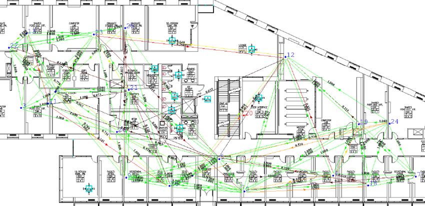
Theorem 1. Two oscillators A and B, governed by RFA Figure 3: Trajectory of the oscillator phases
dynamics, will be driven to synchrony irrespective of their
initial phases.
Proof. Consider two oscillators A and B. Consider the
moment after A has fired and jumped. In the instant after ϕ
~ n+1 = M ϕ
~n (6)
the jump, let φ~ = (φA , φB ) denote the phases of oscillators By the eigendecomposition theorem, we can decompose M
A and B, respectively. The return map R(φ) ~ is defined to as M = V ΛV −1 , where V is the matrix of composed eigen-
be the phases of A and B immediately after the next firing vectors and Λ is a diagonal matrix containing the eigenvalues
of A (which is necessarily after the next firing of B since A of M . To leading non-vanishing order in , the eigenvalues
cannot jump past B1 ) (in Λ) are λ1 = 2 and λ2 = (1+), and the principal eigendi-
We now calculate the return map R(φ). ~ Without loss rections (the rows of V −1 ) are v̄1 = (1, 1) and v̄2 = (0, ).
of generality assume φA < φB . Since A has just fired, B The decomposition allows us to rewrite (6) as
records A’s firing time as φB . Both oscillators move forward
in their cycles until B fires. After B fires, according to our θ~n+1 = Λθ~n (7)
algorithm, B jumps to phase ∆(φB ). In the meanwhile,
A has moved forward a distance 1 − φB , reaching phase where θ~n = V −1 ϕ ~ n is a change-of-basis transformation
φA + 1 − φB , and recording this as B’s last firing time. After that maps all vectors into a new coordinate system spanned
A’s next firing, it jumps to ∆(φA + 1 − φB ), and B is at by the basis B = {v̄1 , v̄2 }. Equation (7) shows us that the
∆(φB )+1−(φA +1−φB ) = ∆(φB )+φB −φA . Substitution of evolution of the system is most simply described in terms
the expression for ∆(φ) and algebraic simplification yields: of B. The system’s evolution along the directions v̄1 and
v̄2 is illustrated in Figure 3. First, all trajectories rapidly
~ n+1 = R(φ
φ ~n ) = M φ
~ n + ~b (3) approach the φA = 0 axis along the vector v̄1 = (1, 1)
since λ1 = 2
1. Upon reaching the axis, trajectories
Here n denotes the cycle number. The vector ~b is defined are repelled away from φ ~ ∗ = (0, 1/2), along the direction
as (e − 1, 0), and the matrix M is defined as v̄2 = (0, ), since λ2 > 1. If a trajectory approaches the
axis from below φ ~ ∗ , it will slide down the axis to the state
e − 1 −(e − 1) ~ = (0, 0). Otherwise, it will climb up to
of synchrony φ
M= (4) ~ = (0, 1), another state of synchrony. Thus φ∗ is a repeller
−1 e φ
Hence the algorithm can be described as a linear dynam- and the oscillators are driven to synchrony, irrespective of
~ where φ~ ∈ [0, 1] × [0, 1]. The unique fixed initial phases. QED
ical system in φ,
point of this dynamical system is easily shown to be:
Rate of synchronization. How quickly the system syn-
chronizes depends on how fast it moves in the v̄2 direc-
~∗ = 0 tion away from φ ~ ∗ before it reaches a state of synchrony.
φ 1 (5)
2 We can estimate the time to synchronization, starting from
~ ∗ both A and B would be exactly half a cycle apart. ~ (0) = (φ(0) , φ(0) ). Given such an initial state, the system’s
φ
At φ A B
We now show that φ ~ ∗ is unstable (i.e.. a ”repeller”) such trajectory will intersect the φA = 0 axis at approximately
(0) (0)
that the phases gets pushed to either (0,0) or (1,1) where δ = φB − φA . The distance from the fixed point grows
the dynamics no longer change. Introducing the change of exponentially fast with eigenvalue λ2 = (1 + ) in the v̄2
variables ϕ ~n − φ
~n = φ ~ ∗ we can rewrite (3) as direction. Let k denote the number of iterations required.
1
Solving λk2 (δ − 12 ) = 12 yields
If A fires and then jumps to φA , then φA ≤ φB for the
following reason: If the phase of B is φB when A reaches
φ = 1, then A must have observed B fire at φx ≥ 1 − φB 1 1 1 1
k= ln( ) ≈ ln( ) (8)
(since B would have fired and then taken a positive jump). ln(1 + ) 2δ − 1 2δ − 1
After firing A takes a jump of φA = ∆(φx ). ∆(x) is always
≤ 1 − x because it is truncated to never cause a jump past Thus, the time to synchrony is inversely proportional to .
the end of the cycle. Therefore φA ≤ 1 − φx ≤ φB .Note that these proofs are very similar to the two os- 6. SIMULATION RESULTS
cillator case for Mirollo and Strogatz, and most likely can We have implemented the Firefly algorithm in TinyOS [4]
be extended to n nodes. However extending these results using the TOSSIM [7] simulator environment. This simula-
to multi-hop topologies requires considerably more sophis- tor has several limitations. It does not model radio delay
ticated analysis [8]. Instead we evaluate the algorithm in correctly, and nor does it take into account clock skew that
simulation for different n and network topologies. occurs from variations in clock crystals in individual wireless
sensors. Despite these limitations, the simulator is useful for
5. EVALUATION TOOLS AND METRICS exploring the parameter space of our algorithm. This can
Both our simulation and testbed experiments output a help us determine optimal parameter settings for the algo-
series of node IDs and firing times. In order to discuss the rithm on a real testbed as well as better understand the
accuracy of the achieved synchronicity, it is necessary to impact of the parameter values on the level of synchronic-
identify groups of nodes firing together. ity achieved. In our simulator experiments, we explore the
For this purpose, we identify sets of node firings that fall impact of varying:
within a prespecified time window. We call each cluster
of node firings a group. Given a time window size w, the 1. Node topology: all-to-all where each node can com-
clustering algorithm outputs a series of firing groups that municate with every other node, and a regular grid
meet two constraints. First, every node firing event must topology where a node can directly exchange messages
fall within exactly one group. Second, groups are chosen to with at most four other nodes.
contain as many firing events as possible. 2. Firing function constant value: ranging from 10-
We define the group spread as the maximum time differ- 1000. Theoretically, the time to synchronize is propor-
ence between any two firings in the group. The time window tional to the firing function constant value.
size w represents the upper bound on the group spread. 3. Number of nodes (n): We examine whether the im-
pact of the firing function constant and node topology
5.1 Evaluation Metrics varies with the number of nodes. The size of the all-
The two evaluation metrics that we are concerned with to-all topologies is varied between 2-20 nodes with 2
involve the amount of time until the system achieves syn- node increments, and grid topologies are varied from
chronicity (if at all), and the accuracy of the achieved syn- 16, 64, to 100 nodes.
chronicity.
All-to-all Topology Results. Figures 4(a) and 5 show
Time To Sync: This is defined as the time that it takes the results of simulations on the all-to-all topology. We
all nodes to enter into a single group and stay within ran simulations for firing function constant values (FFC)
that group for 9 out of the last 10 firing iterations. 10,20,50,70,100,150,300,500,750 and 1000, repeating this com-
The value chosen for the time window w does impact bination for number of nodes ranging from 2-20 in 2 node
the measured time to sync; a very small w will result increments. For each parameter choice, we ran 10 simu-
in a time to sync that is longer than with a larger w, lations using different random seeds to start the nodes at
because it takes longer for all nodes to join a firing different times. Each experiment was run for 3600 seconds
group within a smaller time window. Also, as will of simulation time. Also the time period T = 1sec for all
be discussed in the next sections, the simulator has experiments.
lower time resolution than the testbed hardware which Fig. 4(a) shows the percentage of simulations that syn-
means there is a limit on the accuracy it can achieve. chronized for a selection of parameter values. This percent-
Therefore, for the simulator we set w = 0.1sec and in age represents the fraction of runs that achieved synchronic-
the real testbed we set w = 0.01sec. ity out of the 10 total runs, for a given parameter choice of n
and F F C. We can see that the FFC values displayed in the
50th and 90th Percentile Group Spread: Recall that figure (70,100,300,500 and 750) are fairly reliable since these
the group spread measures the maximum time differ- cases achieved synchronicity in a majority of the simulation
ence between any two events in a firing group. We runs. Most experiments with small firing function constants
wish to characterize the distribution of group spread (10,20,50) did not achieve synchronicity. One likely rea-
for all groups after the system has achieved synchronic- son for this behavior is that small FFC values lead nodes
ity. Although synchronicity may be achieved according to make extremely large jumps, causing them to overshoot
to the time to sync metric above, we wish to avoid mea- (see Section 3.4).
suring group spread while the system is still settling. Fig. 5(a) shows the time to synchronize as a function of
Given the first sync time ts and the time the experi- FFC value and the number of nodes. The graph shows that
ment ends te , we calculate the group spread distribu- most FFC constants work well. The time to sync increases
tion across all groups in the interval [ts + (te −t
2
s)
, te ]. with increasing FFC value but not beyond 400 time periods.
In this way we are measuring the distribution across There is no clear trend with increasing numbers of nodes,
all “tight” groups rather than settling effects. We plot although small FFCs do not work as well with large numbers
the 50th and 90th percentile of the distribution. of nodes. This is possibly because the effect of overshoot is
worsened when there are more neighbors (and thus more
Lastly, we define the Firing Function Constant (FFC) to total firing events per cycle to react to).
be the value 1/, which is the main parameter in the RFA Fig. 5(b) shows the corresponding group spreads. For
algorithm. As discussed in Section 3.4, this parameter limits most FFC values and most n, the 90th percentile group
the response of a node to be at most T /F F C and thus the spread remains the same. The 50th percentile shows a slight
time to synchronize is directly proportional to F F C. increase with increasing FFCs and a slight increase with100 100
4 nodes 16 nodes
8 nodes 64 nodes
80 12 nodes 80 100 nodes
16 nodes
Percentage Synchronized (%)
Percentage Synchronized (%)
20 nodes
60 60
40 40
20 20
0 0
FF 70 FF 100 FF 300 FF 500 FF 750 FF 1000 FF 20 FF 50 FF 100 FF 500
Firing function constant Firing function constant
(a) (b)
Figure 4: Percentage of simulations that achieved synchronicity for different firing function constants and
numbers of nodes. (a) All-to-all topology. Small firing function constants (E.g. 10,20,50,150) did not achieve
synchronicity most of the time. (b) Grid Topology. Experiments with very small firing function constants
(E.g. FFC=10) or very large firing function constants (E.g. > 500) did not achieve synchronicity.
1200
4500
4 nodes 4 nodes
1000
50th and 90th percentile group spread (usec)
8 nodes 8 nodes
4000
12 nodes 12 nodes
16 nodes 16 nodes
3500
800 20 nodes 20 nodes
Time to sync (sec)
3000
600 2500
2000
400
1500
1000
200
500
0 0
FF 70 FF 100 FF 500 FF 750 FF 1000 FF 70 FF 100 FF 500 FF 750 FF 1000
Firing function constant Firing function constant
(a) (b)
Figure 5: All-to-all topology. (a) Time to Sync, which for most cases increases with increasing FFC values.
(b) Group Spread. The solid bars represent the 50th percentile spread, while the error bar indicates the 90th
percentile. For most FFC values, the group spreads remain similar, with a slight increase as the number of
nodes increases
1200
40000
16 nodes 16 nodes
1000 35000
50th and 90th percentile group spread (usec)
64 nodes 64 nodes
100 nodes 100 nodes
30000
800
Time to sync (sec)
25000
600
20000
15000
400
10000
200
5000
0 0
FF 20 FF 50 FF 100 FF 500 FF 20 FF 50 FF 100 FF 500
Firing function constant Firing function constant
(a) (b)
Figure 6: Grid Topology. (a) Time to Sync, which increases with increasing FFC values and network diameter.
(b) Group Spread. The solid bars represent the 50th percentile spread, while the error bar indicates the 90th
percentile. Group spread remains similar over varying FFC values, but increases with network diameter. For
large grids, FFC=500 does synchronize as well, as also shown in Figure 4.increasing numbers of nodes. However, the difference in the
spreads is not large and thus group spreads remain fairly
similar over all parameter values. The error bars for this
data (not shown here) show that there is not much variation
across different experimental runs.
Grid Topology Results. Fig. 4(b) and 6 show the sim-
ulation results for regular grid topologies of 4x4, 8x8, and
10x10 nodes. Fig. 4(a) shows the percentage of cases that
synchronized for a selection of parameter values. The results
show that FFC values in the range of 20-500 almost always
achieve synchronicity in a grid topology.
The behavior of nodes in a grid topology reflects the im- Figure 7: Connectivity Map: The distribution and
pact of network diameter on performance. Fig. 6 (a) shows connectivity of sensor nodes (detailed image at
that large values of the firing function constant increase the http://motelab.eecs.harvard.edu/).
time taken to achieve synchronicity, and that this effect is
more pronounced for larger grids. Larger FFC values im-
ply that nodes make smaller jumps and thus converge to 7.1.1 Network Topology
synchrony more slowly. For a given FFC, the time to sync
We conducted our experiments on the most densely pop-
also increases slightly with network diameter, but not by
ulated floor, with 24 nodes. Statistics on message loss rates
much for the smaller FFC constants. The error bars for the
are calculated periodically and tend to vary over time. Ex-
FFC=500 simulations (not shown here) show that there is
amining the connectivity map and graph shown in Figures
a large variation in time to sync and group spread across
7 and 8, one can see that this is a complex multi-hop topol-
runs, most likely caused by the initial phase distribution of
ogy. The layout of the building produces two cliques of
nodes in the grid which can only be corrected slowly. Bar-
nodes that are connected by high quality links (less than 20%
ring that case, Fig. 6 (b) shows that the group spread does
message loss) and these cliques are connected by only a few
not vary significantly with FFC value. However there does
bridge nodes. Further examination of the cliques shows that
seem to be an increase in spread (i.e. decrease in accuracy)
a large fraction of the links are asymmetric in quality and
for larger grids, indicating that the network diameter may
some nodes (e.g. 2, 26) may have no incoming links of good
have an impact on how well the system can synchronize.
quality. This type of complex topology is representative of
sensor networks distributed in a complex environment.
7. WIRELESS SENSOR NETWORK 7.1.2 Time Stamping with FTSP
TESTBED EVALUATION In order to evaluate the performance of RFA, we need to
Having proven our algorithm correct in simple cases and time stamp the firing messages so that we can determine the
explored the parameter space using TOSSIM, we then tested accuracy with which the firing phases align. However, this
RFA on a real sensor network testbed. The experiments proved to be difficult in our testbed environment. Unlike
carried out on the 24-node indoor wireless sensor network TOSSIM, our sensor nodes do not have access to a global
testbed, show the performance of our algorithm running on clock. Furthermore, since they are distributed throughout
real hardware, with a complex topology, and experiencing the building, there is no single base station that can act as
communication latencies over lossy asymmetric links. The a global observer and provide a common time base [9]. In
table in Figure 10 summarizes our results, showing that RFA an ironic way, evaluating RFA requires an independent and
can rapidly synchronize all the nodes to approx. 100 µsec. accurate implementation of time stamping.
This section is structured as follows. First, we describe To address this difficulty we deployed the Flooding Time
our testbed environment, focusing on the significant ways in Synchronization Protocol (FTSP) [9] described in Section
which the testbed differs from the TinyOS simulator. We 2. FTSP provides nodes access to a stable global clock and
then describe our use of FTSP to provide a common global allows them to time stamp events with precisions reported
time base for nodes participating in our experiments. We in the tens of microseconds. We characterized the errors
then discuss our experiments and results, and compare them in FTSP on our MoteLab topology in the following way.
to our expectation from theory and simulation. Nodes log all firing messages they hear from other nodes
and the time stamp that FTSP assigned to them. For every
7.1 Testbed Environment firing message heard by more than two nodes, we compute
Our experiments ran on MoteLab [16], a wireless sensor the differences between the times that FTSP reported on
network testbed consisting of 24 MicaZ motes distributed each node, taking the maximum difference between any two
over one floor of our Computer Science and Electrical En- stamps. This is only done for messages where FTSP on both
gineering building. The MicaZ motes have a 7.3MHz clock. the sender and receiver reported that the nodes were well-
Each device is attached to a Crossbow MIB600 interface synchronized to the global clock. The cumulative distribu-
backchannel board allowing remote reprogramming and data tion frequency (CDF) of these errors for all of our testbed
logging. Messages sent to the nodes’ serial ports are logged experiments is shown in Figure 9. Note however that the
by a central server. Using this data-logging capability, nodes FTSP errors are only calculated for nodes that are within
report their firing times as well as information about firing one hop of each other, therefore we do not know the error
messages they observe. This information is then used to in FTSP between two arbitrary nodes. Given this caveat,
evaluate the performance of our algorithm, as well as better our results show that FTSP can quickly synchronize nodes
understand its behavior. to within one hop errors of tens of microseconds.26
25
21 4
29
23 28
6 2
11 18
16 5
22 7
9 20
27 19
12
1 24
13
3
Figure 8: Connectivity graph of the nodes on our testbed showing links with better than 80% packet reception.
This reveals two highly-connected subgraphs and a high percentage of asymmetry in link quality.
both locally time stamp and set timers at µsec level resolu-
1
FTSP Errors
tion by multiplexing the SysTime and MicroTimer compo-
0.9
nents onto one hardware counter. The simulator TOSSIM
0.8
provides 4MHz local time stamping through access to its
0.7
internal clock, but no equivalent of the MicroTimer com-
0.6 ponent, forcing us to rely on the standard TinyOS Timer
0.5 component with its millisecond resolution. This limits the
0.4 resolution of the jumps a node can take and therefore the
0.3 algorithm achieves only millisecond accuracy in simulation.
0.2 As we were using the simulator primarily to explore the
0.1 impact of parameter and topology, we felt the lack of preci-
0
1e-06 1e-05 1e-04 0.001 0.01 0.1 1
sion this introduced was acceptable. The higher frequency
FTSP Error (sec)
MicroTimer component is the primary reason that group
spread results from our testbed experiments are much better
than the simulation, which at first would seem surprising.
Figure 9: CDF of one hop FTSP error rates col- 7.2 Performance Evaluation
lected during all of our testbed experiments. FTSP The table in Figure 10 summarizes the results from our
provided the global clock for RFA evaluation. experiments. We conducted four experiments with firing
function constants (FFC) 100, 250, 500 1000.
In each of these experiments the network achieves syn-
The use of FTSP as the global clock impacts our experi- chronicity. In the case with a FFC of 100, the network
mental results in two ways. First, our results are pessimistic is synchronized within 5 minutes, with a group spread of
since their accuracy is limited by the accuracy of time stamp- 131 µsec. As expected from our theoretical and simulation
ing which is likely to be in the 5-10 µsec range. Secondly, studies, the time to synchronize increases with larger fir-
this prevents us from making an objective comparison of ac- ing function constants. The table also shows the 50th and
curacy between FTSP and RFA. In the future, we plan to 90th percentile group spread, and Figure 11 plots the group
use more controlled experimental setups to better evaluate spread CDFs for each of the four FFCs. As we can see they
the accuracy of RFA and compare it to other methods. are striking similar, aligning with our expectations from the-
ory and simulations that group spread does not depend on
7.1.3 Differences From the Simulator the FFC value.
Sensor network devices in a real environment exhibit be- These results are very encouraging, given the caveats on
havior not modeled by TOSSIM. Most significant differences our time stamping and the complexity of the testbed envi-
for our algorithm are (1) communication latencies are un- ronment. However, there are also several features which are
predictable and difficult to measure accurately, (2) links are still unexplained and we plan to investigate these more in
asymmetric and fluctuate over time, and (3) crystal differ- the future. Here we discuss two examples.
ences cause node clocks to tick at different rates. All these One observation from the CDF plot in Figure 11 is that
effects make it difficult for a node to know exactly when an- there seems to be a limit on the achievable group spread of
other node fired, and unlikely that it will hear every firing around 100 µsec. This could be related to FTSP accuracy,
message sent by its neighbors. but it is also affected by clock skew. We expect clock skew
Paradoxically, our testbed is better than TOSSIM in one to impact the accuracy of RFA because the M&S model
very significant way. The sensor node hardware has a high- upon which it is based assumes that nodes agree on a fixed
precision clock and high-precision timer components. A firing period. However, two perfectly synchronized nodes
TinyOS component written for our project allows nodes to will diverge on the very next firing by the amount of driftFFC constant Time to 50th pct 90th pct Mean group from perturbation. However, a more rigorous instrumenta-
sync (sec) spread spread std dev tion and experimentation setup will be required to pinpoint
(µsec) (µsec)
100 284.3 131.0 4664.0 410.4
the causes behind this behavior.
250 343.6 128.0 3605.0 572.2
500 678.1 154.0 30236.0 1327.8
1000 1164.4 132.0 193.0 63.6
8. COMPARISON TO OTHER METHODS
Compared to algorithms such as RBS, TPSN and FTSP[2,
9, 3], the firefly-inspired algorithm represents a radically
Figure 10: Summary of Testbed Results. Four ex- different approach. All of the nodes behave in a simple
periments were run on the 24 node testbed, with dif- and identical manner. There are no special nodes, such as
ferent firing function constants (where F F C = 1/) the root in TPSN or reference node in RBS, that need to
As expected, the time to synchronize increases with elected. A node does not maintain any per-neighbor or per-
FFC. The 50th percentile group spread is similar for link state; in fact it is completely agnostic to the identity of
all four experiments. its neighbors. The algorithm remains the same even if the
topology is multi-hop. There are no network-level datas-
tructures, such as the spanning tree in TPSN, that must
Group Spread CDF
be re-established in case of topology change. As a result
1
100 of these properties, the algorithm is implicitly robust to the
250
0.9 500
1000 disappearance of nodes and links. Lucarelli et al [8] have
0.8
shown that the algorithm works on time-varying topologies;
0.7
our testbed results show that the algorithm performs well
0.6
even with asymmetric, lossy links. The inherent adaptive
0.5
nature of such algorithms is one of the main attractions of
0.4
biologically-inspired approaches.
0.3
Nevertheless, it is not yet clear whether such an algorithm
0.2
will be competitive to algorithms such as TPSN and FTSP,
0.1
in terms of accuracy and overhead, and much work remains
0
1e-05 1e-04 0.001
Group Spread (sec)
0.01 0.1 to be done. In terms of accuracy, RFA achieves 100 µsec
which is significantly less than the reported 10 µsec accu-
racy of FTSP, although as discussed before it is difficult to
make a clear comparison because of the errors caused by
using FTSP as our evaluation clock. We believe that the
Figure 11: CDF of RFA Group Spread. The four
accuracy can be increased to tens of microseconds by elim-
different firing function constants in the testbed ex-
inating errors in our evaluation methodology and by using
periments produce similar levels of synchronicity.
a better optimized MAC-layer delay estimation (as used in
FTSP [9]). However beyond that, the accuracy will still be
limited by clock skew, as discussed in Section 7.2. We intend
that exists in their clocks — introducing an error that is on to investigate models that synchronize both phase and fre-
the order of the crystal accuracy. This causes the nodes to quency, which would eliminate errors cause by clock skew.
constantly readjust their phases. Clock skew also impacts A second shortcoming of RFA is that the communication
the accuracy indirectly when nodes use the message delay overhead is high. In particular, we choose T = 1 sec, unlike
(measured by the sender’s clock) to adjust their own phase. FTSP which has a time period of 30 seconds. Assuming
In the future we plan to investigate the effects of clock skew one could compensate for clock skew, the main limit on T is
more rigorously and look at alternate models of synchroniza- the time taken to synchronize from startup. RFA takes ap-
tion, such as synchronized clapping, where both frequency proximately 200 time periods to synchronize on MoteLab,
and phase are adjusted. which is significantly more than the diameter of the net-
A second observation arises from looking at the group work. On the other hand, the system recovers quickly from
spread over time. We observed that even after tight groups small dispersive events. One option would be to use a sim-
form, occasionally disturbances still occur during the exper- ple mechanism, such as an initial flood, to bring all nodes
iment. We refer to these as dispersive events. Figure 12 (a) to within a small phase difference quickly. Then RFA could
shows an example of a dispersive event where the nodes fall operate at a much lower frequency to tighten the accuracy
out of phase and the system recovers from this impulse over and maintain synchronicity. A different option is to allow
the next few firing periods. Figure 12 (b) shows a differ- nodes to asynchronously backoff, or increase, their time pe-
ent time course with the occurrence of two dispersive events riod in multiples of T depending on whether they observe
which cause the group to spread over approximately 0.1 sec many out-of-phase firing events in their neighborhood. Thus
range. Note that these dispersive events are included in nodes would self-adjust the overhead.
the data in Table 10 and impact the 90th percentile group
spread. Analysis of the information collected during this ex-
periment showed no clear reason for this spurious firing. It 9. CONCLUSIONS AND FUTURE WORK
is unlikely to be caused by the algorithm, since the extent of In this paper we have presented a decentralized algorithm
dispersion is larger than the maximum jump possible given for synchronicity, based on a mathematical model of syn-
the FFC. What is encouraging is that the recovery from the chronicity achieved by biological systems. Our results show
100 msec range dispersive events takes only a few rounds to that even though the theoretical models make simplifying
achieve, thus showing that the system can recover quickly assumptions, this technique still works well and robustly inYou can also read