LEARNING TO REPRESENT ACTION VALUES AS A HYPERGRAPH ON THE ACTION VERTICES - Petar Kormushev
←
→
Page content transcription
If your browser does not render page correctly, please read the page content below
Published as a conference paper at ICLR 2021

L EARNING TO R EPRESENT ACTION VALUES AS
A H YPERGRAPH ON THE ACTION V ERTICES

 Arash Tavakoli ∗                     Mehdi Fatemi                         Petar Kormushev
 Imperial College London              Microsoft Research Montréal          Imperial College London

                                                A BSTRACT

             Action-value estimation is a critical component of many reinforcement learning
             (RL) methods whereby sample complexity relies heavily on how fast a good esti-
             mator for action value can be learned. By viewing this problem through the lens of
             representation learning, good representations of both state and action can facilitate
             action-value estimation. While advances in deep learning have seamlessly driven
             progress in learning state representations, given the specificity of the notion of
             agency to RL, little attention has been paid to learning action representations. We
             conjecture that leveraging the combinatorial structure of multi-dimensional action
             spaces is a key ingredient for learning good representations of action. To test this,
             we set forth the action hypergraph networks framework—a class of functions for
             learning action representations in multi-dimensional discrete action spaces with a
             structural inductive bias. Using this framework we realise an agent class based
             on a combination with deep Q-networks, which we dub hypergraph Q-networks.
             We show the effectiveness of our approach on a myriad of domains: illustrative
             prediction problems under minimal confounding effects, Atari 2600 games, and
             discretised physical control benchmarks.

1       I NTRODUCTION
Representation learning methods have helped shape recent progress in RL by enabling a capacity for
learning good representations of state. This is in spite of the fact that, traditionally, representation
learning was less often explored in the RL context. As such, the de facto representation learning
techniques which are widely used in RL were developed under other machine learning paradigms
(Bengio et al., 2013). Nevertheless, RL brings some unique problems to the topic of representation
learning, with exciting headway being made in identifying and exploring such topics.
Action-value estimation is a critical component of the RL paradigm (Sutton & Barto, 2018). Hence,
how to effectively learn estimators for action value from training samples is one of the major prob-
lems studied in RL. We set out to study this problem through the lens of representation learning, fo-
cusing particularly on learning representations of action in multi-dimensional discrete action spaces.
While action values are conditioned on both state and action and as such good representations of both
would be beneficial, there has been comparatively little research on learning action representations.
We frame this problem as learning a decomposition of the action-value function that is structured in
such a way to leverage the combinatorial structure of multi-dimensional discrete action spaces. This
structure is an inductive bias which we incorporate in the form of architectural assumptions. We
present this approach as a framework to flexibly build architectures for learning representations of
multi-dimensional discrete actions by leveraging various orders of their underlying sub-action com-
binations. Our architectures can be combined in succession with any other architecture for learning
state representations and trained end-to-end using backpropagation, without imposing any change to
the RL algorithm. We remark that designing representation learning methods by incorporating some
form of structural inductive biases is highly common in deep learning, resulting in highly-publicised
architectures such as convolutional, recurrent, and graph networks (Battaglia et al., 2018).
We first demonstrate the effectiveness of our approach in illustrative, structured prediction problems.
Then, we argue for the ubiquity of similar structures and test our approach in standard RL problems.
    ∗
        Correspondence to: Arash Tavakoli .

                                                       1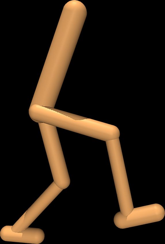
Published as a conference paper at ICLR 2021

Our results advocate for the general usefulness of leveraging the combinatorial structure of multi-
dimensional discrete action spaces, especially in problems with larger action spaces.

2     BACKGROUND
2.1   R EINFORCEMENT LEARNING

We consider the RL problem in which the interaction of an agent and the environment is modelled
as a Markov decision process (MDP) (S, A, P, R, S0 ), where S denotes the state space, A the
action space, P the state-transition distribution, R the reward distribution, and S0 the initial-state
distribution (Sutton & Barto, 2018). At each step t the agent observes a state st ∈ S and produces
an action at ∈ A drawn from its policy π(. | st ). The agent then transitions to and observes the next
state st+1 ∈ S, drawn from P (. | st , at ), and receives a reward rt+1 , drawn from R(. | st , at , st+1 ).
The standard MDP formulation generally abstracts away the combination of sub-actions that are
activated when an action at is chosen. That is, if a problem   has an N v -dimensional action space,
                                                         Nv
                                  v        1 2
each action at maps onto an N -tuple (at , at , . . . , at ), where each ait is a sub-action from the
ith sub-action space. Therefore, the action space could have an underlying combinatorial structure
where the set of actions is formed as a Cartesian product of the sub-action spaces. To make this
                                           .
explicit, we express the action space as A = A1 × A2 × · · · × AN v , where each Ai is a finite set of
sub-actions. Furthermore, we amend our notation for the actions at into at (in bold) to reflect that
actions are generally combinations of several sub-actions. Within our framework, we refer to each
sub-action space Ai as an action vertex. As such, the cardinality of the set of action vertices is equal
to the number of action dimensions N v .
Given a policy π that maps states onto distributions over the actions,     P∞ the discounted sum of future
rewards under π is denoted by the random variable Zπ (s, a) = t=0 γ t rt+1 , where s0 = s, a0 = a,
st+1 ∼ P (. | st , at ), rt+1 ∼ R(. | st , at , st+1 ), at ∼ π(. | st ), and 0 ≤ γ ≤ 1 is a discount factor. The
action-value function is defined as Qπ (s, a) = E[Zπ (s, a)]. Evaluating the action-value function
Qπ of a policy π is referred to as a prediction problem. In a control problem the objective is to find
an optimal policy π ∗ which maximises the action-value function. The thesis of this paper applies to
any method for prediction or control provided that they involve estimating an action-value function.
A canonical example of such a method for control is Q-learning (Watkins, 1989; Watkins & Dayan,
1992) which iteratively improves an estimate Q of the optimal action-value function Q∗ via

                                                                                  0
                Q(st , at ) ← Q(st , at ) + α rt+1 + γ max        0
                                                                      Q(s  t+1 , a  ) − Q(st , at )  ,        (1)
                                                                 a

where 0 ≤ α ≤ 1 is a learning rate. The action-value function is typically approximated using a
parameterised function Qθ , where θ is a vector of parameters, and trained by minimising a sequence
of squared temporal-difference errors
                                                                                2
                            .

                                                             0
                        δt2 = rt+1 + γ max  0
                                               Q θ (st+1 , a   ) − Qθ (st , at )                (2)
                                                 a

over samples (st , at , rt+1 , st+1 ). Deep Q-networks (DQN) (Mnih et al., 2015) combine Q-learning
with deep neural networks to achieve human-level performance in Atari 2600.

2.2   D EFINITION OF HYPERGRAPH

A hypergraph (Berge, 1989) is a generalisation of a graph in which an edge, also known as a
hyperedge, can join any number of vertices. Let V = {A1 , A2 , . . . , AN v } be a finite set repre-
senting the set of action vertices Ai . A hypergraph on V is a family of subsets or hyperedges
H = {E1 , E2 , . . . , EN e } such that
                                       Ej 6= ∅       (j = 1, 2, . . . , N e ) ,                              (3)
                                           e
                                        ∪N
                                         j=1 Ej = V.                                                         (4)
According to Eq. (3), each hyperedge Ej is a member of E = P(V ) \ ∅, where P(V ), called the
powerset of V , is the set of possible subsets on V . The rank r of a hypergraph is defined as the
maximum cardinality of any of its hyperedges. We define a c-hyperedge, where c ∈ {1, 2, . . . , N v },

                                                          2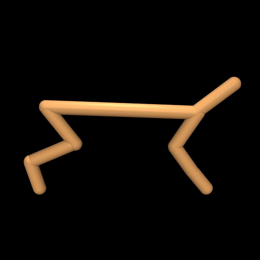
Published as a conference paper at ICLR 2021

Figure 1: (a) A sample hypergraph overlaid on a physical system with six action vertices. (b) An
instance building block of our framework for a sample hyperedge. (c) An architecture is realised by
stacking several building blocks, one for each hyperedge in the hypergraph.

as a hyperedge with cardinality or order c. The number of possible c-hyperedges on V is given by
                            v
the binomial coefficient Nc . We define a c-uniform hypergraph as one with only c-hyperedges. As
a special case, a c-complete hypergraph, denoted K c , is one with all possible c-hyperedges.

3    ACTION HYPERGRAPH NETWORKS FRAMEWORK
We now describe our framework using the example in Fig. 1. Consider the sample physical system of
Fig. 1a with six action vertices (solid circles). A sample hypergraph is depicted for this system with
four hyperedges (dashed shapes), featuring a 1-hyperedge, two 2-hyperedges, and a 3-hyperedge.
We remark that this set of hyperedges constitutes a hypergraph as there are no empty hyperedges
(Eq. (3)) and the union of hyperedges spans the set of action vertices (Eq. (4)).
We wish to enable learning a representation of each hyperedge in an arbitrary hypergraph. To achieve
this, we create a parameterised function UEj (e.g. a neural network) for each hyperedge Ej which
receives a state representation ψ(s) as input and returns as many values as the possible combinations
of the sub-actions for the action vertices enclosed by its respective hyperedge. In other words, UEj
has as many outputs as the cardinality of a Cartesian product of the action vertices in Ej . Each such
hyperedge-specific function UEj is a building block of our action hypergraph networks framework.1
Figure 1b depicts the block corresponding to thev3-hyperedge from the hypergraph of Fig. 1a. We
remark that for any action a = (a1 , a2 , . . . , aN ) from the action space A, each block has only
one output that corresponds to a and, thus, contributes exactly one value as a representation of its
respective hyperedge at the given action. This output UEj ψ(s), aEj is identified by aEj which
denotes the combination of sub-actions in a that correspond to the action vertices enclosed by Ej .
We can realise an architecture within our framework by composing several such building blocks,
one for each hyperedge in a hypergraph of our choosing. Figure 1c shows an instance architecture
corresponding to the sample hypergraph of Fig. 1a. The forward view through this architecture is
as follows. A shared representation of the input state s is fed into multiple blocks, each of which
features a unique hyperedge. Then, a representation vector of size N e is obtained for each action
a, where N e is the number of hyperedges or blocks. These action-specific representations are then
mixed (on an action-by-action basis) using a function f (e.g. a fixed non-parametric function or a
neural network). The output of this mixing function is our estimator for action value at the state-
action pair (s, a). Concretely,
                     .

            Q(s, a) = f UE1 ψ(s), aE1 , UE2 ψ(s), aE2 , . . . , UEN e ψ(s), aEN e

                                                                                        .       (5)

While only a single output from each block is relevant for an action, the reverse is not the case. That
is, an output from a block generally contributes to more than a single action’s value estimate. In
fact, the lower the cardinality of a hyperedge, the larger the number of actions’ value estimates to
which a block output contributes. This can be thought of as a form of combinatorial generalisation.
   1
     Throughout this paper we assume linear units for the block outputs. However, other activation functions
could be more useful depending on the choice of mixing function or the task.

                                                     3
Published as a conference paper at ICLR 2021
Particularly, action value can be estimated for an insufficiently-explored or unexplored action by
mixing the action’s corresponding representations which have been trained as parts of other actions.
Moreover, this structure enables a capacity for learning faster on lower-order hyperedges by receiv-
ing more updates and slower on higher-order ones by receiving less updates. This is a desirable
intrinsic property as, ideally, we would wish to learn representations that exhaust their capacity for
representing action values using lower-order hyperedges before they resort to higher-order ones.
3.1 M IXING FUNCTION SPECIFICATION
The mixing function receives as input a state-conditioned representation vector for each action. We
view these action-specific representation vectors as action representations. Explicitly, these action
representations are learned as a decomposition of the action-value function under the mixing func-
tion. Without a priori knowledge about its appropriate form, the mixing function should be learned
by a universal function approximator. However, joint learning of the mixing function together with
a good decomposition under its dynamic form could be challenging. Moreover, increasing the num-
ber of hyperedges expands the space of possible decompositions, thereby making it even harder to
reach a good one. The latter is due to lack of identifiability in value decomposition in that there is
not a unique decomposition to reach. Nevertheless, this issue is not unique to our setting as repre-
sentations learned using neural networks are in general unidentifiable. We demonstrate the potential
benefit of using a universal mixer (a neural network) in our illustrative bandit problems. However, to
allow flexible experimentation without re-tuning standard agent implementations, in our RL bench-
marks we choose to use summation as a non-parametric mixing function. This boils down the task of
learning action representations to reaching a good linear decomposition of the action-value function
under the summation mixer. We remark that the summation mixer is commonly used with value-
decomposition methods in the context of cooperative multi-agent RL (Sunehag et al., 2017). In an
informal evaluation in our RL benchmarks, we did not find any advantage for a universal mixer over
the summation one. Nonetheless, this could be a matter of tuning the learning hyperparameters.
3.2 H YPERGRAPH SPECIFICATION
We now consider the question of how to spec-
ify a good hypergraph. There is actually not
an all-encompassing answer to this question.
For example, the choice of hypergraph could be
treated as a way to incorporate a priori knowl-
edge about a specific problem. Nonetheless,
we can outline some general rules of thumb.
In principle, including as many hyperedges as
possible enables a richer capacity for discover-
ing useful structures. Correspondingly, an ideal
representation is one that returns neutral val-
ues (e.g. near-zero inputs to the summation
mixer) for any hyperedge whose contribution is
not necessary for accurate estimation of action
values, provided that lower-order hyperedges
are able to represent its contribution. However,
as described in Sec. 3.1, having many mixing Figure 2: (a) A standard model. (b) A class of
terms could complicate reaching a good decom- models in our framework, depicted by the ordered
position due to lack of identifiability. Taking space of possible hyperedges E. Our class of mod-
these into consideration, we frame hypergraph els subsumes the standard one as an instance.
specification as choosing a rank r whereby we
specify the hypergraph that comprises all possible hyperedges of orders up to and including r:
. v
H = ∪r≤N
c=1 K ,
c
(6)
where hypergraph H is specified as the union of c-complete hypergraphs K c . Figure 2b depicts a
class of models in our framework where the space of possible hyperedges E is ordered by cardinality.
On the whole, not including the highest-order (N v ) hyperedge limits the representational capacity of
an action-value estimator. This could introduce statistical bias due to estimating N actions’ values
4Published as a conference paper at ICLR 2021
Figure 3: Prediction error in our illustrative multi-armed bandits with three action dimensions and
increasing action-space sizes. Each variant is run on 64 reward functions in any action-space size.
(a) Normalised average RMS error curves. (b) Average RMS errors at the 400th training iteration.
using a model with M < N unique outputs.2 In a structured problem M < N could suffice, otherwise
such bias is inevitable. Consequently, choosing any r < N v could affect the estimation accuracy in a
prediction problem and cause sub-optimality in a control problem. Thus, preferably, we wish to use
hypergraphs of rank r = N v . We remark that this bias is additional to—and should be distinguished
from—the bias of function approximation which also affects methods such as DQN. We can view
this in terms of the bias-variance tradeoff with r acting as a knob: lower r means more bias but less
variance, and vice versa. Notably, when the N v -hyperedge is present even the simple summation
mixer can be used without causing bias. However, when this is not the case, the choice of mixing
function could significantly influence the extent of bias. In this work we generally fix the choice of
mixing function to summation and instead try to include high-order hyperedges.
4 I LLUSTRATIVE PREDICTION PROBLEMS
We set out to illustrate the essence of problems in which we expect improvements by our approach.
To do so, we minimise confounding effects in both our problem setting and learning method. Given
that we are interested purely in studying the role of learning representations of action (and not of
state), we consider a multi-armed bandit (one-state MDP) problem setting. We specify our bandits
such that they have a combinatorial action space of three dimensions, where we vary the action-space
sizes by choosing the number of sub-actions per action dimension from {5, 10, 20}.
The reward functions are deterministic but differ for each random seed. Despite using a different
reward function in each independent trial, they are all generated to feature a good degree of decom-
posability with respect to the combinatorial structure of the action space. That is to say, by design,
there is generally at least one possible decomposition that has non-zero values on all possible hyper-
edges. See Appendix A for details about how we generate such reward functions.
We train predictors for reward (equivalently, the optimal action values) using minimalist parame-
terised models that resemble tabular ones as closely as possible (e.g. our baseline corresponds to a
standard tabular model) and train them using supervised learning. For our approach, we consider
summation and universal mixers as well as increasingly more complete hypergraphs, specified using
Eq. (6) by varying rank r from 1 to 3. See Appendix A for additional experimental details.
Figure 3a shows normalised RMS prediction error curves (averaged over 64 reward functions) for
two variants of our approach that leverage all possible hyperedges versus our tabular baseline. We
see that the ordering of the curves remains consistent with the increasing number of actions, where
the baseline is outperformed by our approach regardless of the mixing function. Nevertheless, our
model with a universal mixer performs significantly better in terms of sample efficiency. Moreover,
the performance gap becomes significantly wider as the action-space size increases, attesting to the
utility of leveraging the combinatorial structure of actions for scaling to more complex action spaces.
Figure 3b shows average RMS prediction errors at the 400th training iteration (as a proxy for “final”
2
The notions of statistical bias and inductive bias are distinct from one another: an inductive bias does not
necessarily imply a statistical bias. In fact, a good inductive bias enables a better generalisation capacity but
causes little or no statistical bias. In this paper we use “bias” as a convenient shorthand for statistical bias.
5Published as a conference paper at ICLR 2021
Figure 4: Difference in human-normalised score for 29 Atari 2600 games with 18 valid actions,
HGQN versus DQN over 200 training iterations (positive % means HGQN outperforms DQN).
performance) for all variants in our study. As expected, including higher-order hyperedges and/or
using a more generic mixing function improves final prediction accuracy in every case.
Going beyond these simple prediction tasks to control benchmarks in RL we anticipate a general
advantage for our approach, following the same pattern of yielding more significant improvements
in larger action spaces. Indeed, this is if similar structures are ubiquitous in practical RL tasks.
5 ATARI 2600 GAMES
We tested our approach in Atari 2600 games using the Arcade
Learning Environment (ALE) (Bellemare et al., 2013). The action
space of Atari 2600 is determined by a digital joystick with three
degrees of freedom: three positions for each axis of the joystick,
plus a button. This implies that these games can have a maximum
of 18 discrete actions, with many not making full use of the joy-
stick capacity. To focus our compute resources on games with a
more complex action space, we limited our tests to 29 Atari 2600
games from the literature that feature 18 valid actions.
For the purpose of our control experiments, we combine our ap-
proach with deep Q-networks (DQN) (Mnih et al., 2015). The
resulting agent, which we dub hypergraph Q-networks (HGQN),
deploys an architecture based on our action hypergraph networks,
similar to that shown in Fig. 2b, and using the summation mixer.
Given that the action space has merely three dimensions, we in-
stantiate our agent’s model based on a hypergraph including the
seven possible hyperedges. We realise this model by modifying
the DQN’s final hidden layer into a multi-head one, where each
head implements a block from our framework for a respective hy-
peredge. To achieve a fair comparison with DQN, we ensure that Figure 5: Human-normalised
our agent’s model has roughly the same number of parameters median and mean scores across
as DQN by making the sum of the hidden units across its seven 29 Atari 2600 games with 18
heads to match that of the final hidden layer in DQN. Specifically, valid actions. Random seeds are
we implemented HGQN by replacing the final hidden layer of 512 shown as traces.
rectifier units in DQN with seven network heads, each with a sin-
gle hidden layer of 74 rectifier units. Our agent is trained in the same way as DQN. Our tests are
conducted on a stochastic version of Atari 2600 using sticky actions (Machado et al., 2018).
Figure 4 shows the relative human-normalised score of HGQN (three random seeds) versus DQN
(five random seeds) for each game. Figure 5 shows median and mean human-normalised scores
across the 29 Atari games for HGQN and DQN. Our results indicate improvements over DQN on
the majority of the games (Fig. 4) as well as in overall performance (Fig. 5). Notably, these im-
provements are both in terms of sample complexity and final performance (Fig. 5). The consistency
of improvements in these games has the promise of greater improvements in tasks with larger action
spaces. See Appendix B for experimental details, including complete learning curves.
6Published as a conference paper at ICLR 2021
Reacher Hopper HalfCheetah Walker2D Ant
20 3000
2000 1500
2000 3000
Average Score
0 1500
1000 1000
1000 2000
20
0
500
40 500 1000
1000
0 2000 0
60
0 1M 2M 3M 0 1M 2M 3M 0 1M 2M 3M 0 1M 2M 3M 0 1M 2M 3M
Environment Step Environment Step Environment Step Environment Step Environment Step
HGQN (r = 1) HGQN (r = 2) HGQN (r = 3) DQN Rainbow DDPG
Figure 6: Learning curves for HGQN, DQN, and a simplified version of Rainbow in physical control
benchmarks of PyBullet (nine random seeds). Shaded regions indicate standard deviation. Average
performance of DDPG trained for 3 million environment steps is provided for illustration purposes.
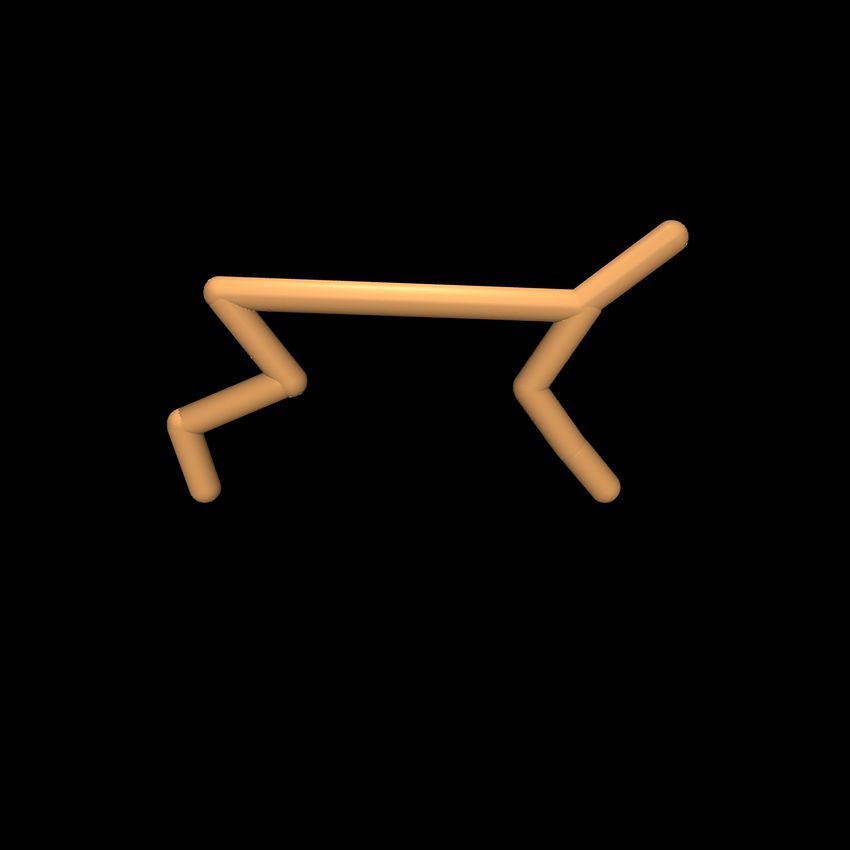
Figure 7: (a) Average (bars) and minimum-maximum (error bars) per-hyperedge representation of
the greedy action over 90000 steps (nine trained rank-3 HGQN models, 10000 steps each). (b) The
actuation morphology of each respective domain is provided for reference.
To further demonstrate the versatility of our approach, we combine it with a simplified version of
Rainbow (Hessel et al., 2018). We ran the resulting agent on the three best and worst-performing
games from Fig. 4. We report our results in Appendix C. Notably, our results show that where HGQN
outperforms DQN most significantly, its combination with the simplified version of Rainbow also
outperforms the corresponding Rainbow baseline.
6 P HYSICAL CONTROL BENCHMARKS
To test our approach in problems with larger action spaces, we consider a suite of physical control
benchmarks simulated using PyBullet (Coumans & Bai, 2019). These domains feature continuous
action spaces of diverse dimensionality, allowing us to test on a range of combinatorial action spaces.
We discretise each action space to obtain five sub-actions per joint. See Appendix D for experimental
details, including network architecture changes for the non-pixel nature of states in these domains.
We ran HGQN with increasingly more complete hypergraphs, specified using Eq. (6) by varying
rank r from 1 to 3. Figure 6 shows the learning curves for HGQN and DQN. In low-dimensional
Reacher and Hopper we do not see any significant difference. However, the higher-dimensional
domains render DQN entirely ineffective. This demonstrates the utility of action representations
learned by our approach. In Ant we only ran HGQN with a 1-complete model as the other variants
imposed greater computational demands (see Sec. 8 for more information).
We provide the average final performance of DDPG (Lillicrap et al., 2016) to give a sense of the
performances achievable by a continuous control method, particularly by one that is closely related
to DQN. Interestingly, HGQN generally outperforms DDPG despite using the training routine of
DQN, without involving policy gradients (Sutton et al., 1999). This may be due to local optimisation
issues in DDPG which can lead to sub-optimal policies in multi-modal value landscapes (Metz
et al., 2017; Tessler et al., 2019). Furthermore, we include the performance of DQN combined with
7Published as a conference paper at ICLR 2021
prioritised replay, dueling networks, multi-step learning, and Double Q-learning (denoted Rainbow† ;
see Hessel et al. (2018) for an overview). The significant gap between the performances of this agent
and vanilla HGQN supports the orthogonality of our approach with respect to these extensions.
In Walker2D we see a clear advantage for including the 2-hyperedges, but additionally including the
3-hyperedges relatively degrades the performance. This suggests that a rank-2 hypergraph strikes the
right balance between bias and variance, where including the 3-hyperedges causes higher variance
and, potentially, overfitting. In HalfCheetah we see little difference across hypergraphs, despite it
having the same action space as Walker2D. This suggests that the 1-complete model is sufficient in
this case for learning a good action-value estimator.
Figure 7 shows average per-hyperedge representation of the greedy action learned by our approach.
Specifically, we evaluated nine trained rank-3 HGQN models using a greedy policy for 10000 steps
in each case. We collected the greedy action’s corresponding representation at each step (i.e. one
action-representation value for each hyperedge) and averaged them per hyperedge across steps. The
error bars show the maxima and minima of these representations. In HalfCheetah the significant
representations are on the 1-hyperedges. In Walker2D, while 1-hyperedges generally receive higher
average representations, there is one 2-hyperedge that receives a comparatively significant average
representation. The same 2-hyperedge also receives the highest variation of values across steps.
This 2-hyperedge, denoted {1, 4}, corresponds to the left and right hips in the agent’s morphology
(Fig. 7b). A good bipedal walking behaviour, intuitively, relies on the hip joints acting in uni-
son. Therefore, modelling their joint interaction explicitly enables a way of obtaining coordinated
representations. Moreover, the significant representations on the 3-hyperedges correspond to those
including the two hip joints. This perhaps suggests that the 2-hyperedge representing the hip joints is
critical in achieving a good walking behaviour and any representations learned by the 3-hyperedges
are only learned due to lack of identifiability in value decomposition (see Sec. 3).
7 R ELATED WORK
Value decomposition has been studied in cooperative multi-agent RL under the paradigm of cen-
tralised training but decentralised execution. In this context, the aim is to decompose joint action
values into agent-wise values such that acting greedily with respect to the local values yields the
same joint actions as those that maximise the joint action values. A sufficient but not necessary
condition for a decomposition that satisfies this property is the strict monotonicity of the mixing
function (Rashid et al., 2018). An instance is VDN (Sunehag et al., 2017) which learns to decom-
pose joint action values onto a sum of agent-wise values. QMIX (Rashid et al., 2018) advances
this by learning a strictly increasing nonlinear mixer, with a further conditioning on the (global)
state using hypernetworks (Ha et al., 2017). These are multi-agent counterparts of our 1-complete
models combined with the respective mixing functions. To increase the representational capacity of
these methods, higher-order interactions need to be represented. In a multi-agent RL context this
means that fully-localised maximisation of joint action values is no longer possible. By relaxing
this requirement and allowing some communication between the agents during execution, coordina-
tion graphs (Guestrin et al., 2002) provide a framework for expressing higher-order interactions in
a multi-agent setting. Recent works have combined coordination graphs with neural networks and
studied them in multi-agent one-shot games (Castellini et al., 2019) and multi-agent RL benchmarks
(Böhmer et al., 2020). Our work repurposes coordination graphs from cooperative multi-agent RL
as a method for action representation learning in standard RL.
Sharma et al. (2017) proposed a model on par with a 1-complete one in our framework and evaluated
it in multiple Atari 2600 games. In contrast to HGQN, their model shows little improvement beyond
DQN. This performance difference is likely due to not including higher-order hyperedges, which in
turn limits the representational capacity of their model.
Using Q-learning in continuous action problems by discretisation has proven as a viable alternative
to continuous control. Existing methods deal with the curse of dimensionality by factoring the action
space and predicting action values sequentially (Metz et al., 2017) or independently (Tavakoli et al.,
2018) across the action vertices. Another approach is to learn a (factored) proposal distribution for
performing a sampling-based maximisation of action values (Van de Wiele et al., 2020). Our work
introduces an alternative approach based on value decomposition and further enables a capacity
for explicitly modelling higher-order interactions among the action vertices. We remark that our
8Published as a conference paper at ICLR 2021
1-complete models can achieve linear time complexity when used with a strictly monotonic mixer
(e.g. summation) by enabling to find the action-value maximising actions in a decentralised manner.
Graph networks (Scarselli et al., 2009) have been combined with policy gradient methods for train-
ing modular policies that generalise to new agent’s morphologies (Wang et al., 2018; Pathak et al.,
2019; Huang et al., 2020). The global policy is expressed as a collection of graph policy networks
that correspond to each of the agent’s actuators, where every policy is only responsible for control-
ling its corresponding actuator and receives information from only its local sensors. The information
is propagated based on some assumed graph structure among the policies before acting. Our work
differs from this literature in many ways. Notably, our approach does not impose any assumptions
on the state structure and, thus, is applicable to any problem with a multi-dimensional action space.
The closest to our approach in this literature is the concurrent work of Kurin et al. (2021) in which
they introduce a transformer-based approach to bypass having to assume a specific graph structure.
Chandak et al. (2019) explored learning action representations in policy gradient methods by a sep-
arate supervised learning process. Other methods have been proposed for learning in large discrete
action spaces that have an associated underlying continuous action representation by using a contin-
uous control method (van Hasselt & Wiering, 2009; Dulac-Arnold et al., 2015). Nevertheless, these
methods do not leverage the combinatorial structure of multi-dimensional action spaces.
8 D ISCUSSION AND FUTURE WORK
We demonstrated the potential benefit of using a more generic mixing function in our bandit prob-
lems (Sec. 4). However, in an informal study on a subset of our RL benchmarks, we did not see any
improvements beyond our non-parametric summation mixer. Further exploration of more generic
(even state-conditioned) mixing functions is an interesting direction for future work. In this case,
comparisons with an action-in baseline architecture would be appropriate to investigate how much
of the advantages of using a hypergraph model may come from sharing the parameters of mixing
function across actions as opposed to modelling lower-order hyperedges.
The requirement to maximise over the set of possible actions limits the applicability of Q-learning
in environments with high-dimensional action spaces. In the case of approximate Q-learning, this
limitation is partly due to the cost of computing the possible actions’ values before an exact maximi-
sation can be performed. Our approach can bypass these issues in certain cases (e.g. when using a
1-complete hypergraph with a strictly monotonic mixer; see Sec. 7 for more information). To more
generally address such issues, we can maximise over a sampled set of actions instead of the entire
set of possible actions (Van de Wiele et al., 2020). An approximate maximisation as such will enable
including higher-order hyperedges in environments with high-dimensional action spaces.
We demonstrated the practical feasibility of combining our approach with a simplified version of
Rainbow. An extensive empirical study of the impact of these combinations as well as combining
with further extensions, e.g. for distributional (Bellemare et al., 2017) and logarithmic RL (van Sei-
jen et al., 2019), is left as future work. Moreover, a better understanding of how value decomposition
affects the learning dynamics of approximate Q-learning could help establish which extensions are
theoretically compatible with our approach.
Much could be done to improve learning in continuous action problems by discretisation. For in-
stance, the performance of our approach could be improved by using exploratory policies that exploit
the ordinality of the underlying continuous action structure instead of using ε-greedy. Moreover,
DDPG uses an Ornstein-Uhlenbeck process (Uhlenbeck & Ornstein, 1930) to generate temporally-
correlated action noise to achieve exploration efficiency in physical control problems with inertia.
Using a similar inductive bias could further improve the performance of our approach in such prob-
lems. A more generally applicable approach which does not rely on the ordinality of the action space
is to use temporally-extended ε-greedy exploration (Dabney et al., 2021). The latter could prove es-
pecially useful in discretised physical control problems as such. Another interesting opportunity is
using a curriculum of progressively growing action spaces where a coarse discretisation can help
exploration and a fine discretisation allows for a more optimal policy (Farquhar et al., 2020).
Code availability The source code can be accessed at: https://github.com/atavakol/
action-hypergraph-networks.
9Published as a conference paper at ICLR 2021
ACKNOWLEDGEMENTS
We thank Ileana Becerra for insightful discussions, Nemanja Rakicevic and Fabio Pardo for com-
ments on the manuscript, Fabio Pardo for providing the DDPG results which he used for benchmarks
in Tonic (Pardo, 2020), and Roozbeh Tavakoli for help with visualisation. A.T. acknowledges finan-
cial support from the UK Engineering and Physical Sciences Research Council (EPSRC DTP). We
also thank the scientific Python community for developing the core set of tools that enabled this
work, including TensorFlow (Abadi et al., 2016) and NumPy (Harris et al., 2020).
R EFERENCES
Martín Abadi, Paul Barham, Jianmin Chen, Zhifeng Chen, Andy Davis, Jeffrey Dean, Matthieu
Devin, Sanjay Ghemawat, Geoffrey Irving, Michael Isard, Manjunath Kudlur, Josh Levenberg,
Rajat Monga, Sherry Moore, Derek G. Murray, Benoit Steiner, Paul Tucker, Vijay Vasudevan,
Pete Warden, Martin Wicke, Yuan Yu, and Xiaoqiang Zheng. TensorFlow: A system for large-
scale machine learning. In Proceedings of the USENIX Symposium on Operating Systems Design
and Implementation, pp. 265–283, 2016.
Joshua Achiam. Spinning up in deep reinforcement learning. https://spinningup.
openai.com, 2018.
Peter W. Battaglia, Jessica B. Hamrick, Victor Bapst, Alvaro Sanchez-Gonzalez, Vinicius Zambaldi,
Mateusz Malinowski, Andrea Tacchetti, David Raposo, Adam Santoro, Ryan Faulkner, Caglar
Gulcehre, Francis Song, Andrew Ballard, Justin Gilmer, George Dahl, Ashish Vaswani, Kelsey
Allen, Charles Nash, Victoria Langston, Chris Dyer, Nicolas Heess, Daan Wierstra, Pushmeet
Kohli, Matthew Botvinick, Oriol Vinyals, Yujia Li, and Razvan Pascanu. Relational inductive
biases, deep learning, and graph networks. arXiv:1806.01261, 2018.
Marc G. Bellemare, Yavar Naddaf, Joel Veness, and Michael Bowling. The Arcade Learning Envi-
ronment: An evaluation platform for general agents. Journal of Artificial Intelligence Research,
47:253–279, 2013.
Marc G. Bellemare, Will Dabney, and Rémi Munos. A distributional perspective on reinforcement
learning. In Proceedings of the International Conference on Machine Learning, pp. 449–458,
2017.
Yoshua Bengio, Aaron Courville, and Pascal Vincent. Representation learning: A review and new
perspectives. IEEE Transactions on Pattern Analysis and Machine Intelligence, 35(8):1798–1828,
2013.
Claude Berge. Hypergraphs: Combinatorics of Finite Sets. North-Holland, 1989.
Wendelin Böhmer, Vitaly Kurin, and Shimon Whiteson. Deep coordination graphs. In Proceedings
of the International Conference on Machine Learning, pp. 2611–2622, 2020.
Greg Brockman, Vicki Cheung, Ludwig Pettersson, Jonas Schneider, John Schulman, Jie Tang, and
Wojciech Zaremba. OpenAI Gym. arXiv:1606.01540, 2016.
Jacopo Castellini, Frans A. Oliehoek, Rahul Savani, and Shimon Whiteson. The representational
capacity of action-value networks for multi-agent reinforcement learning. In Proceedings of the
International Conference on Autonomous Agents and Multi-Agent Systems, pp. 1862–1864, 2019.
Pablo Samuel Castro, Subhodeep Moitra, Carles Gelada, Saurabh Kumar, and Marc G. Bellemare.
Dopamine: A research framework for deep reinforcement learning. arXiv:1812.06110, 2018.
Yash Chandak, Georgios Theocharous, James Kostas, Scott Jordan, and Philip S. Thomas. Learning
action representations for reinforcement learning. In Proceedings of the International Conference
on Machine Learning, pp. 941–950, 2019.
Erwin Coumans and Yunfei Bai. PyBullet: A Python module for physics simulation for games,
robotics and machine learning. https://pybullet.org, 2019.
10Published as a conference paper at ICLR 2021
Will Dabney, Georg Ostrovski, David Silver, and Rémi Munos. Implicit quantile networks for
distributional reinforcement learning. In Proceedings of the International Conference on Machine
Learning, pp. 1096–1105, 2018.
Will Dabney, Georg Ostrovski, and André Barreto. Temporally-extended ε-greedy exploration. In
Proceedings of the International Conference on Learning Representations, 2021.
Gabriel Dulac-Arnold, Richard Evans, Hado van Hasselt, Peter Sunehag, Timothy P. Lillicrap,
Jonathan Hunt, Timothy Mann, Théophane Weber, Thomas Degris, and Ben Coppin. Deep rein-
forcement learning in large discrete action spaces. arXiv:1512.07679, 2015.
Gregory Farquhar, Laura Gustafson, Zeming Lin, Shimon Whiteson, Nicolas Usunier, and Gabriel
Synnaeve. Growing action spaces. In Proceedings of the International Conference on Machine
Learning, pp. 4335–4346, 2020.
Meire Fortunato, Mohammad Gheshlaghi Azar, Bilal Piot, Jacob Menick, Ian Osband, Alex Graves,
Volodymyr Mnih, Rémi Munos, Demis Hassabis, Olivier Pietquin, Charles Blundell, and Shane
Legg. Noisy networks for exploration. In Proceedings of the International Conference on Learn-
ing Representations, 2018.
Xavier Glorot and Yoshua Bengio. Understanding the difficulty of training deep feedforward neural
networks. In Proceedings of the International Conference on Artificial Intelligence and Statistics,
pp. 249–256, 2010.
Carlos Guestrin, Michail Lagoudakis, and Ronald Parr. Coordinated reinforcement learning. In
Proceedings of the International Conference on Machine Learning, pp. 227–234, 2002.
David Ha, Andrew Dai, and Quoc V. Le. Hypernetworks. In Proceedings of the International
Conference on Learning Representations, 2017.
Charles R. Harris, K. Jarrod Millman, Stéfan J. van der Walt, Ralf Gommers, Pauli Virtanen, David
Cournapeau, Eric Wieser, Julian Taylor, Sebastian Berg, Nathaniel J. Smith, Robert Kern, Matti
Picus, Stephan Hoyer, Marten H. van Kerkwijk, Matthew Brett, Allan Haldane, Jaime Fernández
del Río, Mark Wiebe, Pearu Peterson, Pierre Gérard-Marchant, Kevin Sheppard, Tyler Reddy,
Warren Weckesser, Hameer Abbasi, Christoph Gohlke, and Travis E. Oliphant. Array program-
ming with NumPy. Nature, 585(7825):357–362, 2020.
Matteo Hessel, Joseph Modayil, Hado van Hasselt, Tom Schaul, Georg Ostrovski, Will Dabney, Dan
Horgan, Bilal Piot, Mohammad Gheshlaghi Azar, and David Silver. Rainbow: Combining im-
provements in deep reinforcement learning. In Proceedings of the AAAI Conference on Artificial
Intelligence, pp. 3215–3222, 2018.
Wenlong Huang, Igor Mordatch, and Deepak Pathak. One policy to control them all: Shared modular
policies for agent-agnostic control. In Proceedings of the International Conference on Machine
Learning, pp. 8398–8407, 2020.
Diederik P. Kingma and Jimmy Ba. Adam: A method for stochastic optimization. In Proceedings
of the International Conference on Learning Representations, 2015.
Vitaly Kurin, Maximilian Igl, Tim Rocktäschel, Wendelin Boehmer, and Shimon Whiteson. My
body is a cage: The role of morphology in graph-based incompatible control. In Proceedings of
the International Conference on Learning Representations, 2021.
Timothy P. Lillicrap, Jonathan J. Hunt, Alexander Pritzel, Nicolas Heess, Tom Erez, Yuval Tassa,
David Silver, and Daan Wierstra. Continuous control with deep reinforcement learning. In Pro-
ceedings of the International Conference on Learning Representations, 2016.
Marlos C. Machado, Marc G. Bellemare, Erik Talvitie, Joel Veness, Matthew J. Hausknecht, and
Michael Bowling. Revisiting the Arcade Learning Environment: Evaluation protocols and open
problems for general agents. Journal of Artificial Intelligence Research, 61:523–562, 2018.
Luke Metz, Julian Ibarz, Navdeep Jaitly, and James Davidson. Discrete sequential prediction of
continuous actions for deep reinforcement learning. arXiv:1705.05035, 2017.
11Published as a conference paper at ICLR 2021
Volodymyr Mnih, Koray Kavukcuoglu, David Silver, Andrei A. Rusu, Joel Veness, Marc G. Belle-
mare, Alex Graves, Martin Riedmiller, Andreas K. Fidjeland, Georg Ostrovski, Stig Petersen,
Charles Beattie, Amir Sadik, Ioannis Antonoglou, Helen King, Dharshan Kumaran, Daan Wier-
stra, Shane Legg, and Demis Hassabis. Human-level control through deep reinforcement learning.
Nature, 518(7540):529–533, 2015.
Fabio Pardo. Tonic: A deep reinforcement learning library for fast prototyping and benchmarking.
arXiv:2011.07537, 2020.
Fabio Pardo, Arash Tavakoli, Vitaly Levdik, and Petar Kormushev. Time limits in reinforcement
learning. In Proceedings of the International Conference on Machine Learning, pp. 4045–4054,
2018.
Deepak Pathak, Chris Lu, Trevor Darrell, Phillip Isola, and Alexei A. Efros. Learning to control
self-assembling morphologies: A study of generalization via modularity. In Advances in Neural
Information Processing Systems, pp. 2295–2305, 2019.
Tabish Rashid, Mikayel Samvelyan, Christian Schroeder de Witt, Gregory Farquhar, Jakob N. Foer-
ster, and Shimon Whiteson. QMIX: Monotonic value function factorisation for deep multi-agent
reinforcement learning. In Proceedings of the International Conference on Machine Learning,
pp. 4295–4304, 2018.
Franco Scarselli, Marco Gori, Ah Chung Tsoi, Markus Hagenbuchner, and Gabriele Monfardini.
The graph neural network model. IEEE Transactions on Neural Networks, 20(1):61–80, 2009.
Tom Schaul, John Quan, Ioannis Antonoglou, and David Silver. Prioritized experience replay. In
Proceedings of the International Conference on Learning Representations, 2016.
Sahil Sharma, Aravind Suresh, Rahul Ramesh, and Balaraman Ravindran. Learning to factor poli-
cies and action-value functions: Factored action space representations for deep reinforcement
learning. arXiv:1705.07269, 2017.
Peter Sunehag, Guy Lever, Audrunas Gruslys, Wojciech Marian Czarnecki, Vinicius Zambaldi, Max
Jaderberg, Marc Lanctot, Nicolas Sonnerat, Joel Z. Leibo, Karl Tuyls, and Thore Graepel. Value-
decomposition networks for cooperative multi-agent learning. arXiv:1706.05296, 2017.
Richard S. Sutton and Andrew G. Barto. Reinforcement Learning: An Introduction. MIT Press, 2nd
edition, 2018.
Richard S. Sutton, David A. McAllester, Satinder P. Singh, and Yishay Mansour. Policy gradient
methods for reinforcement learning with function approximation. In Advances in Neural Infor-
mation Processing Systems, pp. 1057–1063, 1999.
Arash Tavakoli, Fabio Pardo, and Petar Kormushev. Action branching architectures for deep rein-
forcement learning. In Proceedings of the AAAI Conference on Artificial Intelligence, pp. 4131–
4138, 2018.
Chen Tessler, Guy Tennenholtz, and Shie Mannor. Distributional policy optimization: An alternative
approach for continuous control. In Advances in Neural Information Processing Systems, pp.
1352–1362, 2019.
Emanuel Todorov, Tom Erez, and Yuval Tassa. MuJoCo: A physics engine for model-based control.
In Proceedings of the IEEE/RSJ International Conference on Intelligent Robots and Systems, pp.
5026–5033, 2012.
George E. Uhlenbeck and Leonard S. Ornstein. On the theory of the Brownian motion. Physical
Review, 36(5):823–841, 1930.
Tom Van de Wiele, David Warde-Farley, Andriy Mnih, and Volodymyr Mnih. Q-learning in enor-
mous action spaces via amortized approximate maximization. arXiv:2001.08116, 2020.
Hado van Hasselt and Marco A. Wiering. Using continuous action spaces to solve discrete problems.
In Proceedings of the International Joint Conference on Neural Networks, pp. 1149–1156, 2009.
12Published as a conference paper at ICLR 2021
Hado van Hasselt, Arthur Guez, and David Silver. Deep reinforcement learning with Double Q-
learning. In Proceedings of the AAAI Conference on Artificial Intelligence, pp. 2094–2100, 2016.
Harm van Seijen, Mehdi Fatemi, and Arash Tavakoli. Using a logarithmic mapping to enable lower
discount factors in reinforcement learning. In Advances in Neural Information Processing Sys-
tems, pp. 14134–14144, 2019.
Jianhao Wang, Zhizhou Ren, Beining Han, and Chongjie Zhang. Towards understanding linear
value decomposition in cooperative multi-agent Q-learning. arXiv:2006.00587, 2020.
Tingwu Wang, Renjie Liao, Jimmy Ba, and Sanja Fidler. NerveNet: Learning structured policy with
graph neural networks. In Proceedings of the International Conference on Learning Representa-
tions, 2018.
Ziyu Wang, Tom Schaul, Matteo Hessel, Hado van Hasselt, Marc Lanctot, and Nando de Freitas.
Dueling network architectures for deep reinforcement learning. In Proceedings of the Interna-
tional Conference on Machine Learning, pp. 1995–2003, 2016.
Christopher J. C. H. Watkins. Learning from delayed rewards. PhD thesis, University of Cambridge,
1989.
Christopher J. C. H. Watkins and Peter Dayan. Q-learning. Machine Learning, 8(3):279–292, 1992.
13Published as a conference paper at ICLR 2021
A I LLUSTRATIVE PREDICTION PROBLEMS : E XPERIMENTAL DETAILS
Environment We created each reward function by randomly initialising a hypergraph model with
all possible hyperedges. Explicitly, in each independent trial, we sampled as many values as the
total number of outputs across all possible hyperedges: sampling uniformly from [−10, 10] for the
1-hyperedges, [−5, 5] for the 2-hyperedges, and [−2.5, 2.5] for the 3-hyperedges. This results in
structured reward functions that can be decomposed to a good degree on the lower-order hyperedges
but still need the highest-order hyperedge for a precise decomposition. Next, we generated a random
mixing function by uniformly sampling the parameters of a single-hidden-layer neural network from
[−1, 1]. The number of hidden units and the activation functions were sampled uniformly from
{1, 2, . . . , 5} and {ReLU, tanh, sigmoid, linear}, respectively. Lastly, a deterministic reward for
each action was generated by mixing the action’s corresponding subset of values.
Architecture We used minimalist parameterised models that resemble tabular ones as closely as
possible. As such, our baseline corresponds to a standard tabular model in which each action value
is estimated by a single unique parameter. In contrast, our approach does not require a unique
parameter for each action as it relies on mixing multiple action-representation values to produce an
action-value estimate. Therefore, for our approach we instantiated as many unique parameters as
the total number of outputs from each model’s hyperedges. For any model using a universal mixer,
we additionally used a single hidden layer of 10 rectifier units for mixing the action-representation
values, initialised using the Xavier uniform method (Glorot & Bengio, 2010).
Training Each predictor was trained by backpropagation using supervised learning. We repeatedly
sampled minibatches of 32 rewards (with replacement) to update a predictor’s parameters, where
each training iteration comprised 100 such updates. We used the Adam optimiser (Kingma & Ba,
2015) to minimise the mean-squared prediction error.
The number of hyperedges in our hypergraphs of interest (see Sec. 3.2) can be expressed in terms of
binomial coefficients as
r≤N v
. X Nv
|H| = , (7)
c=1
c
where hypergraph H is specified by its rank r according to Eq. (6). As we discussed in Sec. 3,
each action’s value estimator is formed by mixing as many action-representation values as there are
hyperedges in the model (Eq. (5)). In our simple models for the bandit problems, each such value
corresponds to a single parameter. As such, each learning update per action involves updating as
many parameters as the number of hyperedges. Therefore, to ensure fair comparisons, we adapted
the learning rates across different models in our study based on the number of parameters involved
in updating each action’s value estimate. Concretely, we set a single effective learning rate across
all models in our study. We then obtained each model’s individual learning rate α via
. effective learning rate
α= . (8)
|H|
We used an effective learning rate of 0.0007 in our study. While this achieves the same actual
effective learning rate for both the baseline and our models using the summation mixer, the same
does not hold exactly for our models using a universal mixer. Nonetheless, this still serves as a
useful heuristic to obtain similar effective learning rates across all models. Importantly, the baseline
receives the largest individual learning rate across all other models—especially one that improved
its performance with respect to any other learning rates used by the variants of our approach.
The logic behind the adjustments of learning rate here simply does not hold in the case of high-
capacity, nonlinear models such as those used in our RL benchmarks. Therefore, in our RL bench-
marks we used the same learning rate across all variants.
Evaluation The learning curves were generated by calculating the RMS prediction error across
all possible actions after each training iteration per independent trial.
14Published as a conference paper at ICLR 2021
B ATARI 2600 GAMES : E XPERIMENTAL DETAILS
We based our implementation of HGQN on the Dopamine framework (Castro et al., 2018).
Dopamine provides a reliable open-source code for DQN as well as enables standardised bench-
marking in the ALE under the best known evaluation practices (see, e.g., Bellemare et al. (2013);
Machado et al. (2018)). As such, we conducted our Atari 2600 experiments without any modifi-
cations to the agent or the environment parameters with respect to those outlined in Castro et al.
(2018), except for the network architecture change for HGQN (see Sec. 5). Our DQN results are
based on the published Dopamine baselines. We limited our tests in Atari 2600 to all the games from
Wang et al. (2016) that feature 18 valid actions excluding Defender for which DQN results were not
provided as part of the Dopamine baselines.
The human-normalised scores reported in this paper were given by the formula (similar to van
Hasselt et al. (2016); Dabney et al. (2018))
scoreagent − scorerandom
, (9)
scorehuman − scorerandom
where scoreagent , scorehuman , and scorerandom are the per-game scores (undiscounted returns) for the
given agent, a reference human player, and random agent baseline. We used Table 2 from Wang
et al. (2016) to retrieve the human player and random agent scores.
The relative human-normalised score of HGQN versus DQN in each game (Fig. 4) was given by the
formula (similar to Wang et al. (2016))
scoreHGQN − scoreDQN
, (10)
max(scoreDQN , scorehuman ) − scorerandom
where scoreHGQN and scoreDQN were computed by averaging over their respective learning curves.
Figure 8 shows complete learning curves across the 29 Atari 2600 games with 18 valid actions.
C ATARI 2600 GAMES : A DDITIONAL RESULTS
We combined our approach with a simplified version of Rainbow (Hessel et al., 2018) that includes
prioritised replay (Schaul et al., 2016), dueling networks (Wang et al., 2016), multi-step learning
(Hessel et al., 2018), and Double Q-learning (van Hasselt et al., 2016). We did not include C51
(Bellemare et al., 2017) as it is not trivial how it can effectively be combined with our approach.
We also did not combine with noisy networks (Fortunato et al., 2018) which are not implemented
in Dopamine. We denote the simplified Rainbow by Rainbow† and the version combined with our
approach by HG-Rainbow† .
We ran these agents on the three best and worst-performing games from Fig. 4. We conjecture that
the games in which HGQN outperforms DQN most significantly should feature a kind of structure
that is exploitable by our approach. Therefore, given that our approach is notionally orthogonal
to the extensions in Rainbow† , we can also expect to see improvements by HG-Rainbow† over
Rainbow† . Figure 9 shows the relative human-normalised score of HG-Rainbow† versus Rainbow†
(three random seeds in each case) along with those of HGQN versus DQN from Fig. 4 for these six
games, sorted according to Fig. 4 (blue bars). We see that, generally, the signs of relative scores for
Rainbow† -based runs are aligned with those for DQN-based runs. Remarkably, in Stargunner the
relative improvements are on par in both cases.
This experiment mainly serves to demonstrate the practical feasibility of combining our approach
with several DQN extensions. However, as each extension in Rainbow† impacts the learning process
in certain ways, we believe that extensive work is required to establish whether such extensions are
theoretically sound when combined with the learning dynamics of value decomposition. In fact, a
recent study on the properties of linear value-decomposition methods in multi-agent RL could hint
at a potential theoretical incompatibility with certain replay schemes (Wang et al., 2020). Therefore,
we defer such a study to future work.
Figure 10 shows complete learning curves across the six select Atari 2600 games.
15Published as a conference paper at ICLR 2021
Figure 8: Learning curves in 29 Atari 2600 games with 18 valid actions for HGQN and DQN.
Shaded regions indicate standard deviation.
16You can also read