Is there only one way out of in-work poverty? Difference by gender and race in the US - Emanuela Struffolino Zachary Van Winkle - WZB Bibliothek

Emanuela Struffolino
Zachary Van Winkle

Is there only one way out of in-work poverty?
Difference by gender and race in the US

Discussion Paper
SP I 2019–601
January 2019

Research Area
Dynamics of Social Inequality
Research Group
Demography and Inequality

Copyright remains with the author(s).

Discussion papers of the WZB serve to disseminate the research results of
work in progress prior to publication to encourage the exchange of ideas and
academic debate. Inclusion of a paper in the discussion paper series does not
constitute publication and should not limit publication in any other venue.
The discussion papers published by the WZB represent the views of the
respective author(s) and not of the institute as a whole.
Emanuela Struffolino, Zachary Van Winkle
Is there only one way out of in-work poverty? Difference by gender and
race in the US
Discussion Paper SP I 2019–601
Wissenschaftszentrum Berlin für Sozialforschung (2019)

Affiliation of the authors:

Emanuela Struffolino
WZB Berlin Social Science Center
Zachary Van Winkle
University of Oxford and Nuffield College

Abstract

Is there only one way out of in-work poverty? Difference by gender and race in the
US

by Emanuela Struffolino and Zachary Van Winkle

The persistency of in-work poverty during the last decades challenges the idea that employment
is sufficient to escape poverty. Research has focused on the risk factors associated with in-work
poverty, but scholars know little about individuals’ experiences after exiting it. The Sequence
Analysis Multistate Model procedure is applied to three high-quality longitudinal data sources
(NLSY79, NLSY97, and PSID) to establish a typology of employment pathways out of in-work
poverty and estimate how gender and race are associated with each pathway. We identify five
distinct pathways characterized by varying degrees of labor market attachment, economic
vulnerability, and volatility. White men are most likely exit in-work poverty into stable
employment outside of poverty, while Black men and women likely remain vulnerable and at-
risk of social exclusion as well as recurrent spells of in-work poverty. Gender and race
differences persist even after controlling for labor market related characteristics and family
demographic behavior.

Keywords: Gender, Race, In-Work Poverty, Sequence Analysis, Event History Analysis

                                                                                               3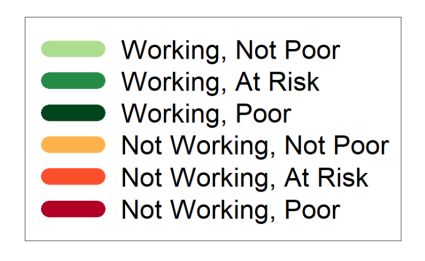

INTRODUCTION

Understanding how individuals successfully escape in-work poverty is central for stratification

and life course research. The working poor, employed individuals who live in households with

incomes below the poverty threshold1, represent a worrisome phenomenon that can engender

social exclusion (Brady et al. 2010). However, individuals’ experiences of in-work poverty vary

considerably. For some individuals, working and being poor is a long-lasting condition, while

for others in-work poverty is a short and sporadic event. Besides the duration of in-work

poverty, some individuals experience multiple, recurring spells of in-work poverty. Similarly to

poverty (Bane and Ellwood 1986; Duncan et al. 1993; Fouarge and Layte 2005; Stevens 1994),

frequent in-work poverty can exacerbate social inequality between social groups that can have

spill-over effects on other life domains. This is of special interest in the United States, where the

primary segment of the labor market is difficult to access for women and individuals from

minority groups. Not holding a stable and protected job not just inhibits chances for upward

mobility, but also exposes these groups to a higher risk of in-work poverty. Most importantly,

the intersection between gender and race has been found to be crucial for the interplay between

both employment and family life (e.g. Aisenbrey and Fasang 2017).

Since the mid-1980s, scholarship on poverty has focused on the temporal dynamics of poverty

spells, i.e. duration and patterns, (Bane and Ellwood 1986; Leisering and Leibfried 1999), but has

recently been enriched by life-course accounts of how family and employment transitions

trigger poverty (Dewilde, 2003; Vandecasteele, 2010). In contrast, most research on the working

poor (see Kenworthy and Marx [2018] for a review) has studied either the association between

in-work poverty and individual factors, e.g. education and family structure, ascriptive

characteristics, e.g. gender and race, or macro-level factors that shape the prevalence of in-

work poverty across countries (e.g., Crettaz and Bonoli 2011; Filandri and Struffolino 2018;

Lohmann and Crettaz 2018). The few longitudinal accounts of in-work poverty study the

probability of entering and exiting the working poor as a function of changes in employment

status and family structure (e.g., Vandecasteele and Gieselmann [2018] for the UK). A recent

contribution adopting a life-course perspective on the US demonstrates that the associations

between family demographic transitions, e.g. entering parenthood and marriage, and the

probability of in-work poverty vary starkly across individuals’ life courses (Van Winkle and

Struffolino 2018). However, understanding the temporal dynamics of how individuals not just

enter but also successfully exit in-work poverty are conducive to informing theory and

1     See      https://www.census.gov/data/tables/time-series/demo/income-poverty/historical-poverty-
thresholds.html for historical thresholds.

                                                                                                   4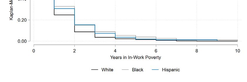

designing effective anti-poverty policies. Yet we do not know how frequent it is to leave in-

work poverty. Further, we do not know about the pathways of employment and economic

wellbeing that individuals take after exiting in-work poverty and whether they differ across

social groups.

This paper aims at filling these gaps and addresses three research questions: First, what

pathways out of an in-work poverty episode exist in the US? Specifically, we assess the

heterogeneity of employment and economic wellbeing trajectories following transitions out of

in-work poverty. This thick description (Abbott 2016) is needed, because scholars lack empirical

knowledge on whether individuals and their households tend to escape in-work poverty

permanently or rather regress into in-work poverty again. Second, to what extent are pathways

out of in-work poverty associated with gender and race? This allows us to gage if and to what

extent gender and race are linked with more or less successful pathways out of in-work

poverty. Third, are gender and race differences in the pathways out of in-work poverty

attributable to average differences in individual characteristics? Particularly, we attempt to

account for the associations between gender and race, and pathways out of in-work poverty

with composition differences in labor market related characteristics and family demographic

behavior.

This paper presents the first substantive application of a novel methodological approach: the

Sequence Analysis Multistate Model (SAMM) procedure (Studer, Struffolino, and Fasang 2018).

SAMM enhances our understating of how time-constant and time-varying individual and

household characteristics are associated with different sequences of events following

transitions out of in-work poverty at any point of the life course. SAMM brings together two

methodological traditions in life course sociology: sequence analysis for the study of holistic life

course patterns and event history analysis for the study of the probability and the timing of life

course transitions. To construct and analyze employment and economic wellbeing trajectories

following in-work poverty spells, we combine three panel data sources – the 1979 and 1997

National Longitudinal Surveys of Youth (NLSY79 and NLSY97) as well as the Panel Study of

Income Dynamics (PSID). Our observational window is therefore exceptionally ample, ranging

between age 18 to 50 from 1968 to 2011 for cohorts born between 1930 and 1984.

Our findings are the first to demonstrate the heterogeneity of pathways out of in-work poverty:

immediate or progressive recovery from in-work poverty, continuous vulnerability, cyclical in-

work poverty, and impoverished unemployment. Further, our results highlight persistent

differences by gender and race in the probability to exit in-work poverty through more and less

advantaged pathways. For example, we show that white men most likely to exit in-work poverty

                                                                                                  5

into stable employment outside of poverty, while Black men and women tend remain at-risk of

poverty outside of employment and often regress into additional spells of in-work poverty.

These gender and race differences persist even after controlling for labor market related

factors, i.e. educational attainment, work experience, and occupational group, as well as family

demographic behavior, i.e. parental home leaving, fertility, and marital union and dissolution.

Our results have important implications for theories and concepts surrounding in-work

poverty. As is the case for poverty (Duncan et al. 1993), the static dichotomy between the

“working poor” and the “working non-poor” is misleading. Our approach shows that one can

account for varying degrees of labor market attachment, economic vulnerability, and volatility

only when looking at individual experiences as they unfold over time. Further, we demonstrate

that standard approaches that do not consider how individual pathways unfold over the years

following in-work poverty mask important gender and race inequalities. Our results indicate

that behavioral theories in poverty research are not adequate to explain how gender and race

differences arise after in-work poverty spells have ended.

TRENDS IN-WORK POVERTY IN THE UNITED STATES

Both great fluctuation and stability characterize the prevalence of in-work poverty in the

United States across the last fifty years. The standard approach to measure poverty in the US

relies on an absolute threshold, which is a function of household composition and is adjusted

yearly for inflation. For example, the federal poverty limit for a single adult in 2018 was

$12,140 before taxes and government transfers and $23,900 for a household with three

members.2 In-work poverty in the US is commonly defined as individuals over age 16 that have

been employed for at least 27 weeks over the year and whose household income lies below the

federal poverty line. This measure contrasts with the relative poverty approach, adopted for

example by Eurostat, which considers individuals whose equivalized household income is below

60% of the national median as poor.3

2 The January 2018 poverty guidelines are calculated by taking the 2016 Census Bureau's poverty
thresholds and adjusting them for price changes between 2016 and 2017 using the Consumer Price Index
(CPI-U) (https://aspe.hhs.gov/poverty-guidelines).
3 EUROSTAT considers individuals who worked at least 7 months, or approximately 28 weeks, as employed
and defines equivalized household incomes using the modified OECD scale below 50-66% of the median as
at risk of poverty. The choices concerning the number of hours or weeks of work to identify workers, what
type of income or benefit should be considered to determine the poverty status, and where to set the
threshold between poor and non-poor remain subject of lively debates (Crettaz 2013). A general agreement
exists on the fact that the unit of analysis has to be the household, especially when aiming at lifting

                                                                                                       6

Absolute and relative poverty stem from different research traditions and definitions of

poverty. Absolute poverty thresholds are defined based on the costs needed to purchase the

minimum amount of goods that are deemed necessary for survival (Sen 1994). As the term

absolute implies, the amount of goods and their cost may remain constant over time, even if

average incomes increase. For example, the US absolute poverty threshold is set approximately

as three times the cost of a minimum food diet in 1963 adjusted for inflation to current prices.

Relative poverty thresholds take a deprivation approach to poverty. In this tradition,

impoverished individuals are at risk of social exclusion if they do not command enough

resources to participate in activities and achieve the standard of living that is customary in

their society (Townsend 1979).

Figure 1 displays the proportion of employed individuals that live in households under the

absolute and relative poverty thresholds and their 95 percent confidence intervals between

1971 and 2018 by gender and race. The left panel presents information for men and the right for

women. There are six trends shown within each panel: the share of white (black line), Black

(blue line), and Hispanic (green line) individuals that are employed, but live in households under

the absolute poverty threshold are presented as solid lines and those under the relative poverty

threshold are shown as dashed lines. Individuals are considered to be employed if they worked

27 or more weeks in the previous year. Households are under the absolute poverty threshold if

their gross household income is below the US Census Bureau poverty threshold. In contrast, the

relative poverty threshold is based on the national income distribution of a given year.

Households with a net equivalized household income below 60 percent of the median are

considered to be under the relative poverty threshold.

[here Figure 1: Proportion of Employed Men and Women in Absolute and Relative Poverty by Race in
                                   the United States, 1971-2018]

As shown in Figure 1, the proportion of employed white men and women in absolute and

relative poverty has remained remarkably stable between the 1970s and 2010s. On average,

nearly 3 percent of white working men and 4 percent of white working women live in

households below the federal poverty limit. At its highest point, approximately 4.5 percent of

white women and 4 percent of white men in work lived in poverty following the early 1980’s

individuals out of poverty by increasing the number of earners (Filandri and Struffolino 2018; Lohmann
and Marx 2018; Thiede, Lichter, and Sanders 2015).

                                                                                                    7

recession. Relative in-work poverty rates are higher, but similarly stable for white men and

women, roughly 9 and 10 percent, respectively.

The share of employed Black and Hispanic men and women that are poor is considerably higher

and more variable across time compared to white men and women. In fact, absolute in-work

poverty rates for Blacks and Hispanics are more similar to the relative in-work poverty rates of

white men and women. While the share of working Black and Hispanic men in poverty was

similar during the 1970s, these trends began to diverge during the 1980s. In 1971,

approximately 10 percent of employed Hispanic and Black men lived in absolute poverty.

Following the passage of the Personal Responsibility and Work Opportunity Act in 1996, well

over 13 percent of Hispanic working men lived in households under the federal poverty limit

and over 30 percent lived in households under the relative poverty threshold, compared to 24

percent in 1971. In-work absolute and relative poverty rates decreased for Black men, reaching

a low of 4 and 17 percent, respectively, in the year 2000.

In contrast to men, in-work poverty rates for Black and Hispanic women converged by the mid-

1990s. Before then, working Black women were more likely to be poor than Hispanic women

during the 1970s and 1980s. In 1971, 16 and 31 percent of employed Black women lived in

households under the absolute and relative poverty thresholds, compared to 7 and 18 percent

for Hispanic women. By 1996, 10 percent of both Black and Hispanic women lived in households

under the federal poverty limit and 28 percent under the relative poverty limit. Those rates

have since changed only to a small degree.

Besides gender and race, other individual and household characteristics have been found to be

associated with an increased risk of in-work poverty (Kenworthy and Marx 2018; U.S. Bureau of

Labor Statistics 2016). Having less than high school education, working part-time, and being

between age 25-43 are important individual predictors of in-work poverty. Household-related

characteristics, e.g. living in a household with children, being the sole breadwinner, and living

in a rural area, increase the risk of in-work poverty by restricting earnings opportunities.

Interestingly, in-work poverty rates by houshehold composition have not changed substantially

between the 1990 and 2010 (Thiede, Sanders, and Lichter, 2018), despite increases in the

aggregate generosity of the US welfare system4 (Spar 2006). A potential explaination is that

welfare support over the last 30 years increased for the disabled and the elderly, while it

decreased for single mothers and their children as well as for families with the lowest incomes

(Danziger 2010; Moffitt 2015).

4 This holds true both when considering social insurance and welfare programs separately and together
with other programs introduced between 1935 and 1996 (see Moffitt [2015] for a review).

                                                                                                   8

BACKGROUND

Life Course Research on Poverty

In this section, we discuss the development of poverty theories that bring a life course approach

to stratification research. In the following section, we then discuss how those approaches might

apply to research on in-work poverty. Cross-sectional studies on poverty tend to underestimate

the rise in the risk of poverty (Sandoval, Rank, and Hirsch 2009). Variation in annual in-work

poverty levels are not only generated by period events, e.g. recessions, but also by changes in

population structure. For example, factors with a stable cross-sectional risk of in-work poverty

may become more widespread across the population, e.g. single parenthood or separation

(Brady, Finnigan, and Hübgen 2017). Most importantly, cross-sectional trends may mask

important shifts in the prevalence of in-work poverty over the life course, e.g. across age

groups. Extending the previous example, the risk of entering in-work poverty associated with

entering parenthood may strengthen across the life course. Therefore, the prevalence of in-

work poverty would increase as the average age at first birth increases.

(Rowntree 1901) recognized over a century ago that poverty should be considered longitudinally

as it emerges and persists at different stages of the life course. Two streams of sociological

literature have embraced this idea: First, classical studies on poverty have adopted a

longitudinal perspective incorporating time as crucial dimension (Bane and Ellwood 1986;

Duncan et al. 1993; Fouarge and Layte 2005; Stevens 1994). These studies highlight that poverty

is specifically located in time and individual biographies (Leisering and Liebfried 1999). This

approach argues that life courses are institutionalized by the welfare state and that poverty

emerges from the exposure to normatively defined, non-insured social risks. Second, the life-

course approach (Elder, 1998; Elder & Rockwell, 1979) emphasizes that life-courses are

multidimensional and unfold in specific historical and social contexts. Life course sociologists

argue that the temporal dynamics of events and transitions in different life domains as well as

how these domains mutually affect one another are dependent on contextual factors at the

family and societal level. For example, the transition onto the labor market and the transition

into marriage were tightly linked during the mid-20th century. This was a time when stable,

gainful and lifetime employment following high school was widespread in the US, which

allowed couples to leave home and found families earlier than their parents and their children.

A recently developed approached, the political economy of the life course (Dewilde 2003),

bridges these two streams by considering how initial advantages and disadvantages accumulate

over time (Dannefer 2003; Merton 1968). Specifically, this approach extends the idea that the

                                                                                                  9

welfare state, the market, and the family shape individuals’ life courses and locate them in

specific social groups. Stratification occurs not only between individual life courses, but also

within them. Therefore, it is essential to analyze trajectories of economic wellbeing as they

unfold over time. To date, most of the empirical research adopting a life course approach has

focused on education, family, and employment trajectories. Although poverty is a relatively rare

event, it should be included as an additional life course dimension for two reasons: First,

economic wellbeing, specifically poverty, has long lasting consequences for other domains.

Second, the direction and the strength of the association between poverty and family dynamics

depend on the phase of the life course at which family transitions occur (Daly 2018; Sandoval et

al. 2009; Settersten and Mayer 1997).

Studies that embrace this perspective generally analyze only at the risk and the timing of

entering and exiting poverty multiple times over a given observational window. These studies

attribute permanent or recurrent poverty spells to durable individual and household

characteristics or to “state dependence”. State dependence refers to the higher likelihood of

experiencing a spell in a specific state (in-work poverty) in the future just because of prior spells

in that state. According to this perspective, slipping into poverty once has scarring effects as it

triggers processes that make future poverty more likely, such as demoralization, habituation,

stigmatization, and depreciation of human capital (Ayllón 2013; Cappellari and Jenkins 2004;

Valletta 2006). However, these studies tend to analyze poverty spells as a series of isolated life

course events and consider the likelihood do being poor at time t+1 given poverty at time t. This

limits our understanding of the temporal dynamic of poverty. (Arranz and Cantó 2012) argue

that researchers should study individual poverty trajectories that account for both poverty and

non-poverty spells to better estimate the aggregate intertemporal poverty risk.

Extending a Life Course Perspective to In-Work Poverty

We adopt and extend this approach to in-work poverty: we argue that in-work poverty needs to

be studied longitudinally as a life course process. Moreover, we propose a typology of relevant

states that combines individual labor market status and household economic hardship to

identify differences in pathways after exiting from in-work poverty to go beyond the dichotomy

poor/non-poor.

First, the temporal dynamics of in-work poverty require that researchers pay attention to how

different degrees of disadvantage in terms of economic wellbeing and labor market attachment

are located along the life course. However, to the best of our knowledge, the few studies that use

longitudinal data to consider how in-work poverty risks develop over the life course share the

                                                                                                  10

same limitations as those focusing on poverty. Recent evidence on the US shows that critical

family demographic transitions, e.g. leaving the parental home, union formation and

dissolution, as well as parenthood, are associated with the probability of belonging to the

working poor (Van Winkle and Struffolino 2018). Further, the strength of these associations

varies across the life course and tend to be stronger for women than men. (Giesselmann 2015)

finds that while in-work poverty is more common among workers entering the labor market in

Germany, those at later stages of their career are more susceptible to in-work poverty in the UK.

Vandecasteele and Gieselmann (2018) estimate the risk of entering and exiting in-work poverty

in the UK and conclude that being in in-work poverty seems to be rather transitory and occurs

at specific phases of the life course. No research has gone beyond estimating the risk of entering

and exiting in-work poverty to consider the pathways experienced by individuals once they

successfully exit an in-work poverty spell. Further, there is no research on whether differences

in these pathways exist across social groups.

Second, focusing solely on the risk of entering or exiting in-work poverty (being the alternative

states a generic in/out in-work poverty dichotomy) masks important elements for theory on in-

work poverty dynamics. Adopting this dichotomous definition of the outcome allows for

identifying only patterns of cyclical in-work poverty or persistent disadvantage in in-work

poverty. Accounting for the actual experience of individuals requires, instead, linking the exit

from in-work poverty to alternative states that signify different degrees of income

vulnerability and labor market attachment. In other words, exiting in-work poverty has to be

conceptualized as a process that can lead to different possible mid-term outcomes.

We extend previous propositions (Filandri and Struffolino 2013; Vandecasteele and Gieselmann

2018) and define a typology of relevant states that combines individual labor market status and

household economic hardship. Figure 2 displays possible states along these two dimensions

between which individuals and households can move over time. On the one hand, an individual

can exit in-work poverty through an improvement in economic wellbeing associated with

his/her labor market participation. Depending on the increase in economic wellbeing,

households are either lifted well above the poverty line or remain at-risk-of poverty. In the

latter case, the intermediate status implies high levels of vulnerability. This is important,

because vulnerability is a weakening process. The lack of resources exposes individuals not only

to the negative consequences related to relative poverty, but also inhibits their recovery or

their ability to take advantage of opportunities to recover when they occur (Spini, Bernardi, and

Oris 2017). On the other hand, exiting in-work poverty can occur through the transition to

unemployment while remaining in poverty. In this case, individuals slip into a state of social

                                                                                               11

exclusion. Employment is considered as the one of the necessary factors to prevent social

exclusion, which is understood as being severely materially deprived and living in a household

with a very low work intensity (Eurostat 2018). Also in this case, an intermediate state of living

in a household at risk-of-poverty while being unemployed represents a vulnerable condition,

because unemployment increases the risk of social exclusion.

Referring to social exclusion/inclusion implies adopting a dynamic approach: social exclusion is

a process that emerges as a consequence of multiple factors associated with the persistence of

unemployment and poverty over time (Atkinson 1998; Negri and Saraceno 2000; Paugam 1998).

Therefore, we argue that our typology has high heuristic potential when applied to the study of

longitudinal dynamics of in-work poverty that goes beyond classifying individuals and

households at specific time points.

           [here Figure 2: Individual Labor Market Status & Household Economic Status]

As we are the first to examine pathways out of in-work poverty, we refrain from formulating

specific expectations about how these processes look like empirically. However, the following

longitudinal pathways could be characterized by stability in one state or by multiple transitions

between several states. For example, precarious pathways out of in-work poverty may lead to

stability within non-poor employment after having been at risk of poverty for a number of

years or may lead back to in-work poverty within a short time.

EXPECTATIONS

Differences in Pathways Out of In-Work Poverty by Gender & Race

The US labor market is highly segmented in a primary labor market, which provides stable

employment relationships and chances for upward mobility, and a secondary labor market,

which is characterized by short-term contracts and frequent periods of unemployment (Berg

and Kalleberg 2001; Griffin, Kalleberg, and Alexander 1981; Kalleberg and Sorensen 1979).

Individuals belonging to the primary labor market segment are more likely to leave in-work

poverty towards non-poor employment, while those in the secondary segment may never

completely escape in-work poverty.

Numerous studies have documented that men are more likely to be employed within the

primary sector, while women are commonly employed in the secondary sector or do not

                                                                                               12

participate on the labor market (Reid and Rubin 2005). This is especially the case for Black and

Hispanic women, who are more likely to experience low prestige careers often interrupted by

unemployment and inactivity (Aisenbrey and Fasang 2017). In light of these differences, we

expect that pathways out of in-work poverty are stratified by gender and race (H1). For example,

pathways out of in-work poverty for men, especially for white men, could be characterized by

stable employment outside of poverty, while pathways out of in-work poverty for women,

especially for Black and Hispanic women, might entail multiple transitions in and out of the

labor market and persistent poverty.

Accounting for Gender & Race differences

Similarly to poverty (see Brady [forthcoming] for a recent review), theoretical explanations for

in-work poverty refer to behaviors, structure, and politics. We explore two mechanisms

stemming from behavioral theoretical explanations of poverty. The first mechanism refers to

the accumulation of resources over time that are associated with labor market participation,

while the second associates poverty to family demographic behavior. Specifically, we extend

these explanations to consider if compositional differences between groups account for gender

and race differences in pathways out of in-work poverty.

The first approach links poverty with resources that individuals command to avoid labor market

disadvantage and life course. Educational attainment, occupational position, and work

experience are considered the most important labor market related resources. In the US, those

with less human-capital related resources are more likely to regress into poverty or have

difficulties re-entering the labor market if they have exited it (Daly and Valletta 2006; Valletta

2006; Worts, Sacker, and McDonough 2010). Further individuals in lower skilled occupational

groups are more likely to experience unemployment and those with more employment

interruptions are less likely to be re-hired (e.g., Gangl 2004).

Average differences in the level of labor market related resources could generate disparities in

pathways out of in-work poverty between gender and racial groups. Blacks and Hispanics tend

to be less educated than whites, hold more precarious jobs, and have less high-quality work

experience (Aisenbrey and Fasang 2017; Ryan and Siebens 2012), which decreases their chances

to leave in-work poverty successfully. During the mid-20th century, men were more educated

than women. However, the education gender gap has tightened and even reversed in recent

decades, women may experience more advantageous pathways out of in-work poverty. Overall,

we expect that gender and race differences in labor market resources account for gender and race

differences in pathways out of in-work poverty (H2).

                                                                                               13

The second approach concerns family demographic behavior, especially leaving the parental

home, entering parenthood as well as union formation and dissolution. While marriage has a

protective function and shields individuals from in-work poverty, separation and entering

parenthood increase the risk of in-work poverty (Thiede et al. 2018; Van Winkle and Struffolino

2018). Leaving the parental home is a poverty-risk factor (Aassve et al. 2007), due to the scarce

amount of resources available when young adults transition onto the labor market. Fertility

transitions as well as union formations and dissolutions affect both the number of potential

earners in the household, but also the economic needs of households (e.g., Hübgen 2018; Uunk

2004).

Again, average differences in family demographic behavior may produce gender and race

disparities in pathways out of in-work poverty. Compared to whites, Black men and women are

more likely to leave the parental home early, enter parenthood early and outside of marriage

(Sweeney and Raley 2014; Wu and Wolfe 2001), as well as form and dissolve a marital union

compared to whites (Bulanda and Brown 2007; Sweeney and Phillips 2004). As for gender, Van

Winkle and Struffolino (2018) show that marriage had a protective function against in-work

poverty for women, while separation increased it across the life course. Parenthood was instead

positively associated with in-work poverty mostly for women at early stages of the transition to

adulthood. Therefore, we expect gender and race differences in family demographic behavior to

account for gender and race differences in pathways out of in-work poverty (H3).

DATA & METHODS

Data

To test our hypotheses, we combine data from three high quality data sources – the 1979 and

1997 National Longitudinal Surveys of Youth (NLSY79 and NLSY97) as well as the Panel Study of

Income Dynamics (PSID). It is necessary to combine data sources to realize a sufficient number of

observations that exit in-work poverty. The NLSY795 consists of 12,686 respondents born

between 1957 and 1964 that were first interviewed in 1979. The NLSY976 sample consists of

8,948 respondents born between 1980 and 1984 that were first interviewed in 1997. While the

NLSY79 and NLSY97 are nationally representative cohort panels, the PSID is a nationally

5 The NLSY79 survey is sponsored and directed by the U.S. Bureau of Labor Statistics and conducted by the
Center for Human Resource Research at The Ohio State University. Interviews are conducted by the
National Opinion Research Center at the University of Chicago.
6 The NLSY97 survey is sponsored and directed by the U.S. Bureau of Labor Statistics and conducted by the
National Opinion Research Center at the University of Chicago, with assistance from the Center for Human
Resource Research at The Ohio State University.

                                                                                                      14

representative household panel. The PSID7 sampled approximately 18,000 individuals within

5,000 households in 1968, with occasional refreshment samples. All three studies continued to

collect economic, sociological and demographic information annually, however currently all

three studies are collected on a biennial basis, starting in 1994 for the NLSY79, 1997 for the

PSID, and 2011 for the NLSY97.

Individual employment trajectories

We construct trajectories for respondents as sequences using annual information on labor

market attachment, household income, and household size. To define our sequence states, we

cross-tabulate labor market status with the poverty status of the respondent’s household. As in

Figure 2, in any given observation period, a respondent can either be “working and not poor”

(WNP), “working and at-risk of poverty” (WAR), “working and poor” (WP), “not working and not

poor” (NWNP), “not working and at-risk of poverty” (NWAR), or “not working and poor” (NWP).

We consider respondents to be employed if they worked over 20 hours a week averaged over the

previous year. This corresponds with working full-time for at least 26 weeks or working part-

time for a full year. Respondents that worked under 20 hours a week averaged over the past

year are defined as not working. The relative poverty threshold is defined as 60 percent of the

median net equivalized household income. Therefore individuals are “working and at-risk of

poverty” if they were employed for at least an average of 20 hours in the previous year and

command household incomes under the relative poverty threshold. Respondents that are

working, but have household incomes over the relative poverty threshold are characterized as

“working and not poor”. Conversely, respondents that are not working and live in households

under the relative poverty threshold are “not working and at-risk of poverty”. We use the US

Census Bureau poverty thresholds to define our absolute poverty thresholds. Note that these

thresholds also vary by household composition. Therefore, working individuals with gross

household incomes under the absolute poverty threshold are defined as “working and poor”, and

those not working then as “not working and poor”. Incorporating both the relative and absolute

poverty thresholds when defining our sequence states allow us to identify the cross-sections of

poverty and employment status conceptualized in Figure 2. For example, “not working and poor”

corresponds to social exclusion, “not working and at-risk of poverty” to the danger of social

7 The collection of data used in this study was partly supported by the National Institutes of Health under
grant number R01 HD069609 and R01 AG040213, and the National Science Foundation under award
numbers SES 1157698 and 1623684. We use an amended version of the WZB-PSID code for data preparation
generated by David Brady and Ulrich Kohler.

                                                                                                        15

exclusion, and those “working and at-risk of poverty” as being characterized by considerable

vulnerability.

We only use annually collected information between ages 18 and 50 to create our sequences, i.e.

excluding data after 1994 for the NLSY79, 1997 for the PSID, and 2011 for the NLSY97. The

maximum sequence length is 16 years up to age 37 for the NLSY79, 14 years up to age 31 for the

NLSY97, and 27 years up to age 50 for the PSID. Our combined sample consists of 37,925

sequences (see Table A1 for descriptive statistics on the study samples).

Methods

We combine approaches from sequence analysis (SA) and event history analysis (EHA) to

empirically identify pathways out of in-work poverty and estimate how the probability of

exiting through those pathways varies by gender and race. EHA and SA are commonly portrayed

as stemming from two different – and even opposing – traditions of life course research (Billari

2005). EHA is concerned with the timing of transitions, such as the age of first birth, and seeks

to identify the probability or hazard of those transitions. SA is interested in trajectories that

consist of a longitudinal series of categorical states, such as employment life courses, and aims

to identify patterns of sequential equivalence. While EHA developed out of a stochastic data

modeling culture, SA is embedded within the tradition of narrative positivism that makes no

assumptions about data generation.

In the field of life-course sociology, EHA has been used in numerous studies on school-to-work

and work-to-retirement transitions, transitions to parenthood as well as marriage and

separation. Since its introduction to the social sciences by Andrew Abbott in the 1980s (Abbott

and Forrest 1986; Abbott and Hrycak 1990), SA has become an established method to study life

course patterns, especially family, education, employment, and retirement trajectories. For our

research question, EHA and SA by themselves are insufficient, because our aim is to estimate

how time-varying factors affect the probability of following a specific pathway after the end of

an episode in in-work poverty. We therefore use sequence analysis multistate models (SAMM), a

stepwise procedure that allows the study of the relationship between time-varying covariates

and the hazard of following distinct trajectories of categorical states following a given transition

(Studer, Stuffolino, and Fasang 2018). SAMM enables us to 1) empirically identify pathways out

of in-work poverty, 2) estimate the associations between gender and race with each pathway out

of in-work poverty, and 3) estimate the extent that these associations are attenuated by labor

market related characteristics and family demographic behavior. The SAMM procedure consists

of five steps, which are discussed in detail below.

                                                                                                 16

Step I: Identifying Subsequences Out for In-Work Poverty

The first step consists of the extraction of subsequences from individuals’ sequences. A

subsequence is a sequence of consecutive states of a given length that begins with a given

transition and is at least one state shorter than the original sequence. Subsequences enable

researchers to isolate trajectories that immediately following a given transition. Our

subsequences begin with a transition out of the state “working and poor” and are five years

long. Therefore, each sub-sequence we extract begins with the state “working and poor”

followed by the next four states observed.

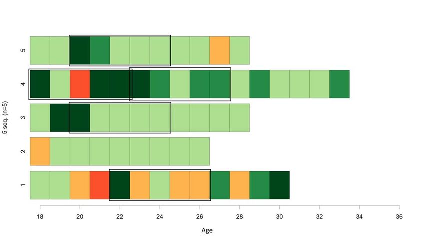
                       [here Figure 3: Example of subsequences’ extraction]

An example of the extraction of five subsequences beginning with a transition out of in-work

poverty from four sequences of varying lengths is displayed in Figure 3. The third sequence is

relatively simple, consisting of one year “working and not poor” at age 18, followed by two

years “working and poor”, and ending at age 28 after 8 years of “working and not poor”. We can

extract one subsequence from this sequence starting from the third time point, “working and

poor”, followed by the next four time points, “working and not poor”. Similarly, we can extract

one subsequence from sequence 1 and 5. In sequence 5, the extracted subsequence also begins

with the third state, “working and poor”, but is followed by one year “working and at-risk” and

then three years “working and not poor”. The subsequence extracted from sequence 1 is more

complex, with one year of “not working and not poor”, followed by one year “working and not

poor” and finishing with two years “not working and not poor”. Notice that the last state

observed in sequence 1 is “working and poor”. However, this cannot be the beginning of a sub-

sequence as we do not observe a transition out of in-work poverty or four additional years of

observation. Finally, we are able to extract two subsequences from sequence 4, because we

observe 2 transitions out of in-work poverty. The first subsequence begins at age 18 and ends

with two years of in-work poverty at ages 21 and 22. The second subsequence starts

immediately after at age 23 with a second transition out of in-work poverty. Therefore,

individual sequences can provide multiple subsequences that may even overlap with one

another. Note that we cannot extract any subsequences from sequence 2, as in-work poverty is

not experienced at any point. Therefore, this individual will not contribute to the analyses

discussed further below. In total, we extract 7,337 subsequences with a length of 5 years that

begin with a transition out of the state “working and poor”.

                                                                                            17

Step II: Calculating Dissimilarities between Subsequences

We calculate a pairwise distance matrix between subsequences using the longest common

substring (LCS) distance measure.8 We choose LCS over other sequence distance measures, such

as dynamic hamming distance or optimal matching with substitution costs, because it

emphasizes ordering as opposed to timing in sequences (Studer and Ritschard 2016). This is

important, because our subsequences are relatively short and there is relatively little variance

in the timing of events across subsequences.

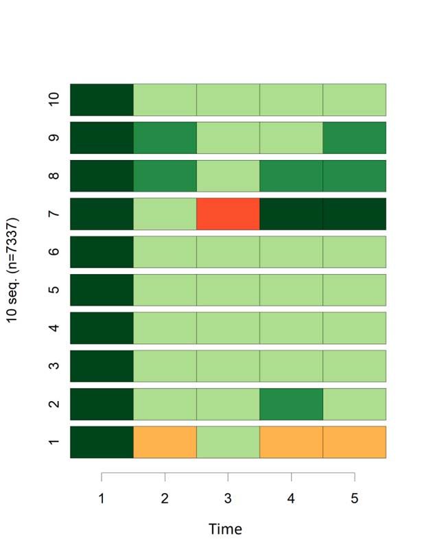
                         [here Figure 4: Alignment of subsequences at time t]

LCS distances are calculated in four steps: First, the subsequences that were extracted in step I

above are aligned as displayed in Figure 4. This means that all subsequences begin with the state

“working and poor” at time 1. The following states are then located at time 2, 3, 4, and 5. In the

second step, the substrings for each subsequence are generated. Substrings contain all the

elements, i.e. single states and an order of states without durations, within a given subsequence

that can be obtained by deleting any element within that sequence. Third, the number of

substrings that every subsequence pair share is quantified as a count metric. That count reflects

the similarity of each subsequence pair. In a fourth and final step, this count is transformed to

reflect dissimilarity.

Step III: Clustering Subsequences

In our next step, we apply a cluster analysis on the set of subsequences using the LCS distance

matrix. We use the partitioning around medoids (PAM) clustering algorithm that separates an

initial set of sequences in subgroups characterized by the highest possible within-group

homogeneity and between-group heterogeneity (Studer 2013). Medoids are representative

sequences that have the smallest dissimilarity to the other sequences of the cluster they belong

to. We choose a five cluster solution after a close consideration of both the average width

silhouette (AWS) values and substantive reasons. The AWS value for the three, four, and five

clusters solution is 0.39, 0.28, and 0.29 respectively: we opted for a five-cluster partition as it

8 Note that LCS stands for the longest common subsequence rather than the longest common substring. We
use the term substring to avoid confusion.

                                                                                                   18

allows us to isolate clusters that are not simply characterized by one single state but rather by

more pronounced dynamics between states.

Step IV: Mixed Effects Competing Risks Cox Hazard Regressions

Besides identifying pathways out of in-work poverty, the aim of this paper is to estimate gender

and race differences in these pathways and to account for these differences. To this end, we use

the clusters as the dependent variables in mixed effects Cox hazard regressions with competing

risks. These models extend upon simple Cox hazard regressions in two ways: First, this strategy

allows us to model multiple failure types. Specifically, we can estimate the gender and race

differences in the hazard of exiting in-work poverty through each cluster or pathway identified

in step three. Second, mixed effects Cox hazard regressions retrieve unbiased standard errors

for multiple failures or censors per individual. In particular, these models correct for frailty, i.e.

or individual’s differential propensity to exit in-work poverty and to contribute multiple

failures to the estimation sample.

Simple Cox hazard regressions model the time specific hazard or risk of a given event for an

individual based on a baseline hazard function and a number of predictor variables and

coefficients. In our case, process time begins when an individual enters in-work poverty and

ends upon that individual’s exit out of in-work poverty or until the individual is no longer

observed, i.e. right censored. To reduce the problem of left censoring, we exclude individuals

whose fist observation is in the state “working and poor”. The hazard of exiting in-work poverty

into any other state λ, at a specific time t, for a given individual j, is modelled as:

                                                                                                   1

where the individual predictor variables and their coefficients Xjβ, are multiplicatively related

to the baseline hazard of exiting in-work poverty into any other state λ0. The multiplicative

relatedness between the baseline hazard and the covariates, or the proportional hazards

assumption, is integral for the non-parametric form of the model. In this model, the values of

individual covariates are free to vary over time. Note that the model as formulated in equation 1

allows only one failure type and only one failure per subject, but can be extended to include

multiple failures per subject by estimating clustered standard errors.

For our purposes, we need to extend this model to account for multiple failure types and failures

per subject. To accomplish this, we estimate a number of mixed effects Cox models with

competing risks. Here the time specific hazard λ(t), of a failure type k, for the ith failure or censor

of an individual j, is modelled as:

                                                                                                    19

,                                                                                              2a

where the individual predictors and their coefficients Xijβ, are multiplicatively related to the

baseline hazard specific to the failure type λ0k. In this case, process time begins when an

individual enters in-work poverty and ends when an individual exits in-work poverty through

the failure type, i.e. cluster. As an example, consider the subsequences displayed in Figure 4

again. The observations, i.e. the subsequences, from sequence 1 and 5 spend only one year in the

state “working, poor” before exiting. Therefore, they are at risk of exiting in-work poverty

through a given pathway for one year. In contrast the second observation, i.e. subsequence, from

sequence 4 spends three years within the state “working, poor” before exiting. Equation 2a is

therefore not only modeling the probability to exit in-work poverty through a specific cluster,

but also the time spent within the state “working and poor” before exiting.

The estimated standard errors are corrected for multiple failures and censored spells from

individuals by incorporating individual random intercepts bj, into the regression models:

  ~    0,                                                                                        2b

As is the case in applications with linear mixed random effects models, the variance of our

random intercepts is assumed to be normally distributed with a mean of zero and a variance of

σ2, as displayed in equation 2b.

Analytical strategy

Our analytical strategy proceeds in three steps related to three questions: 1) how persistent is

in-work poverty, 2) how do individuals exit in-work poverty, and 3) what gender and race

differences are there in how individuals exit in-work poverty? First, simple Cox hazard

regressions as displayed in equation 1 are used to model the hazard of exiting in-work poverty

into any state. This allows us to establish a baseline for how common it is to exit in-work

poverty in the US and whether in-work poverty is a long- or short-term event in peoples’ lives.

Further, we estimate gender and race differences in the hazard to exit in-work poverty and to

what extent those differences are accounted for by compositional differences. The analytical

sample for these analyses consist of 7,289 individuals that contribute 9,578 spells of in-work

poverty after list wise deletion of observations with missing values on our independent

variables discussed below. Of those 9,578 spells, we observe 8,883 exits out of in-work poverty.

Before list wise deletion, our sample consists of 13,398 observations spells and 12,406 exits.

In our second step, we address how individuals exit in-work poverty. Specifically, we discuss the

empirical pathways out of in-work poverty that we identified using cluster analysis on the

                                                                                                 20

5,828 subsequences we extracted in steps I above. When discussing these clusters, we pay special

attention to their qualitative differences and their distribution across the sample.

Finally, use mixed effects Cox hazard regressions with competing risks to establish what gender

and race differences in the pathways out of in-work poverty exist and whether we can account

for those differences. To this end, we estimate three stepwise competing risks Cox hazard

regressions as in equations 2a: Model 0 is a baseline model that estimates gender and race

differences in the hazard of exiting in-work poverty through each pathway we identified. In

model 1, we include indicators for educational attainment, work experience, and occupational

group. Educational attainment is measured in years of education corresponding with the highest

grade completed. Work experience reflects the cumulative number of years employed since age

18. We use a revised version of the one-digit ISCO scheme to group occupation into i)

management and professionals, ii) technical, sales, and administrative support, iii) service, iv)

farming, fishing, craft, and production, v) operators, fabricators, and laborers, and vi) military

service or out of the labor force. Model 2 includes three family demographic indicator variables:

1) whether the respondent lives in the parental home, 2) whether the respondent is childless,

has one child, two children, or three or more children, and 3) whether the respondent has never

been married, is married, or is separated or divorced. All models are adjusted for respondents’

year of birth, age, age-squared, and the study. Further, all covariates that vary across time, e.g.

educational attainment or the number of children, are entered into the models as time-varying

covariates. Before list wise deletion of missing values on our core independent variables, we

observe 5,828 individuals that contribute 6,990 subsequences, i.e. exits out of in-work poverty,

and 10,859 spells of in-work poverty. After list wise deletion our sample drops to 4,344

individuals, 4,887 subsequences, and 7,590 spells.

Note that our race variable distinguishes between whites, Blacks, and Hispanics. We exclude

Native Americans, Asian Americans, and Pacific Islanders to ensure that the white category

comprises only individuals of European or Western descent or ancestry. This is important to

ensure that our categories do not combine groups that are not equally privileged (compared to

whites) or not equally marginalized (compared to Blacks and Hispanics). We include gender and

race as a single categorical variable in all models, i.e. white men, white women, black men, etc.,

to adequately account for intersectionalities between gender and race. We have conducted

several robustness checks to ensure that our results are not driven by decisions on modeling or

other factors, such as the inclusion of weighting schemes, the differentiation between never

married and cohabiting, the length of subsequences, and selection into in-work poverty. A

thorough discussion of these robustness checks can be requested to the authors.

                                                                                                21

RESULTS

Cox Regression Results: Exiting In-Work Poverty

Before examining the pathways out of in-work poverty, it is important to ascertain whether in-

work poverty represents a short phase in individuals’ lives or is more persistent. To this end, we

estimate four Cox regressions on the hazard of exiting in-work poverty. The coefficients of

these models represent changes in the hazard to leave the state “working and poor” regardless

of the following state. These results are available upon request.

 [here Figure 5: Kaplan-Meier Survival Estimates on Exiting In-Work Poverty by Gender and Race]

In the baseline models, we see that Black and Hispanic men as well as Black women have a lower

propensity to exit in-work poverty compared to white men. The survival curves by gender and

race displayed in Figure 5 demonstrate that differences emerge relatively early, but diminish

after 4 years within in-work poverty. Nearly 80 percent of white men exit in-work poverty

within one year, while only 70 percent of Black and Hispanic men and only 60 percent of Black

women escape in-work poverty within a year. These differences, in the magnitude of roughly 10

percentage points, remain until the fifth year within in-work poverty. Nearly all individuals,

regardless of gender or race, exit in-work poverty after six years. These differences, although

small and attenuated slightly, remain statistically significant even after controlling for both

labor market related factors and family demographic behavior.

In sum, we do observe some gender and race disparities in the timing and propensity to exit in-

work poverty. Further, these disparities cannot be completely attributed to compositional

differences. However, the gender and race differences in the hazard of exiting in-work poverty

give us no indication of what happens to individuals in the years following their exit out of in-

work poverty. A fast exit out of in-work poverty does not necessarily mean recovery, for

example, if individuals exit the labor force, but continue to live in impoverished households or

regress into another spell of in-work poverty.

Cluster Analysis Results: Pathways Out of In-Work Poverty

What pathways do individuals follow after transitioning out of in-work poverty? The results of

our second analysis step, sequence and cluster analysis on subsequences beginning with a

                                                                                               22

transition out of in-work poverty, are displayed as relative frequency sequence plots in Figure 6

(see Fasang and Liao [2014] for relative sequence plots). Each plot depicts 100 subsequences that

represent their cluster.9 As can be seen, every subsequence begins in the state “working and

poor”. We extract a five-cluster solution: 1) immediate recovery, 2) progressive recovery, 3)

continuous vulnerability, 4) cyclical in-work poverty, and 5) impoverished non-employment.

  [here Figure 6: Relative Frequency Sequence Plots of Pathways Out of In-Work Poverty Clusters]

The cluster “immediate recovery”, compromising 18.5 percent of all subsequences, is

characterized by a direct exit out of in-work poverty into stable employment outside of poverty.

Compared to all other clusters, this is the most advantageous pathway out of in-work poverty.

Individuals in our largest cluster, 37.6 percent of all subsequences, tend to achieve employment

outside of poverty. However, rather than an immediate transition into stable employment, men

and women in the “progressive recovery” cluster experience an instable transition out of in-

work poverty. Although most experience spells of employment while being at-risk of poverty,

others temporarily exit the labor market or regress back into in-work poverty. Approximately

17 percent of transitions out of in-work poverty are characterized by “continuous

vulnerability”. While these individuals remain employed and exit absolute poverty, they

continue to live in households that are at constant risk of poverty.

Two of our clusters, “cyclical in-work poverty” and “impoverished non-employment”, represent

extremely turbulent and precarious pathways out of in-work poverty. Slightly over 16 percent

of all subsequences are characterized by a regression back into in-work poverty within four

years. Many of these individuals escape in-work poverty by exiting the labor market or slipping

out of absolute poverty. Our final cluster, compromising just under 11 percent of all transitions

out of in-work poverty, regress not into in-work poverty, but remain either at-risk of poverty

or in absolute poverty outside of the labor market. As we expected, there is no single pathway

out of in-work poverty, but rather a number of pathways characterized by different degrees of

economic vulnerability, labor market attachment, and volatility.

The composition of our cluster varies by gender and race as well as labor market related factors

and family demographic behavior. Descriptive statistics on these clusters by sample are

available upon request. Although the “immediate recovery” cluster contains roughly 18.5

9 Summary statistics on the representativeness of each subsequence and the plots as a whole are available
upon request.

                                                                                                       23