Lab 5: Asteroid Rotational Periods
←
→
Page content transcription
If your browser does not render page correctly, please read the page content below
Astronomical Laboratory 29:137 Fall 2007

Lab 5: Asteroid Rotational Periods
This laboratory involves designing
an observational program to
determine the rotational period of
an asteroid with previously
unknown period. The observations
will be taken using the Rigel
Telescope, and the student will
perform differential photometry to
make the first measurement of the
period. As part of this project, all
students need to acquire basic
competence in Unix O/S and Talon
tools for image analysis and differential photometry.

The best web reference for this project is the CALL website (Collaborative
Asteroid Lightcurve Link):

http://www.minorplanetobserver.com/astlc/

The scientific goals of this project are:

   1. Confirm a known asteroid period.

       Identify an asteroid near opposition with a period in the range 4 hr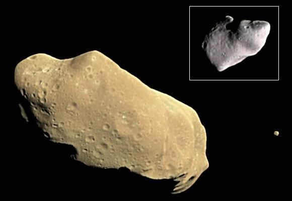
Astronomical Laboratory 29:137 Fall 2007

              Make a quick plot using gnuplot. Read the data into Logger Pro) fit
              a best-fit sine curve.

   2. Measure and publish new rotational period:

Determine the rotational period of (at least one) previously unknown asteroid
using the same observing scheme as above. To determine which asteroids are
near opposition and that do not have measured rotational period, see the CALL
list of potential lightcurve targets for Oct-Dec 2007:

         http://www.minorplanetobserver.com/astlc/targets_4q_2007.htm

          a. In order to ensure a successful detection, you will need to chose at
             least several candidates (since many asteroids have either very
             long periods or very small magnitude differences).

          b. The period must be determined accurately: A full period is required.
             If you obtain only a partial period, you need to re-observe and
             combine datasets.

          c. The results must be submitted to the Minor Planet Center (see
             CALL website for details). Do not submit without review by the
             instructor!

   3. To learn a bit about Unix, the lingua franca of scientific operating systems.

          Background and Theory

Asteroids typically are irregularly shaped (e.g. 243 Ida above, with its satellite
Dactyl) so that as they rotate, the effective cross sectional area changes as
viewed from a Earth-base observer. Hence by observing the light curve as the
asteroid rotates, the rotational period can by determined. Knowledge of the
rotation period allows us to determine the distribution of angular momentum per
unit mass in various asteroid families, which in turn is an important clue in
understanding the origin of the solar system.

 While more than 100,000 asteroids are
now catalogued, only about 1% have
measured rotational periods. Typical
rotational periods are 5-15 hours, so it
often possible to obtain an entire light
curve in a single evening for an asteroid
near solar opposition. The amplitude of
the light curve varies with size, with the
large asteroids having smaller light
variations since they tend to be more
nearly spherical. For asteroids with
diameters less than 100 km, the light
Astronomical Laboratory 29:137 Fall 2007 curve amplitude is typically 0.1-0.3 magnitude or even larger depending on the degree of irregularity of the asteroid's shape. Determining the rotational period of an asteroid involves careful monitoring of the apparent magnitude of the asteroid over a large enough time interval to determine the period unambiguously. This will typically involve several nights of observing using aperture photometry with nearby field stars as magnitude references. In the figure above, the asteroid 1147 Stavropolis was observed at the Iowa Robotic Observatory in a single night. Each data point is separated by ~15 minutes. The light curve has a characteristic double-peaked sinusoidal signature, with a rotational period 5.0 0.5 hours. The calibration star light curve should ideally be flat – in this example, the photometric error was ~0.03 magnitudes RMS. An introductory web page on asteroids is at: http://www.solarviews.com/eng/asteroid.htm Comprehensive summary data on asteroids are located at the Minor Planet Center (MPC): http://cfa-www.harvard.edu/iau/mpc.html the European Asteroid Research Network (EARN) at: http://129.247.214.46/archives.html and the Asteroid Observing Services at Lowell Observatory: http://asteroid.lowell.edu/ A very nice site with plenty of images and a few movies of an asteroid fly-by is at: http://www.solstation.com/stars/asteroid.htm An excellent reference on rotational periods, including observing lists of potential targets as a function of season, is the ‘Collaborative Asteroid Lightcurve Link’ (CALL) at: http://www.MinorPlanetObserver.com/astlc/default.htm
Astronomical Laboratory 29:137 Fall 2007

          Observing strategy

A. Choosing a asteroid with a known rotational period

          a. For the first part (asteroid with known period), use Megastar to find
             bright asteroids near opposition. Then compare the asteroids near
             opposition with the Harris list.

          In Megastar:

                  i. First make sure date/time and location are set correctly
                     (Options. Tucson is close enough).
                 ii. Find the Sun (short-cut key L = locate). Opposition
                     coordinates will be 12h different in RA, flip sign of
                     declination. Center on this position (short-cut key C =
                     coords)
                iii. Set field of view to about 15 deg (shortcut key F)
                iv. Turn off stars (Stars/remove), turn on asteroids
                     (SolarSys/Filters – no comets, asteroid limit 14), Label by
                     number (Solarsys/Label Options/Number)
                 v. Compte current positions (Solarsys/Compute asteroid
                     positions), display asteroids (Solarsys check Asteroids). You
                     should see something like this:
Astronomical Laboratory 29:137 Fall 2007
vi. Now start comparing asteroids in the field to the Harris list to
find a suitable asteroid
b. Prepare an observing request using the Rigel telescope schedule
request web form and your assigned observer’s code. For the
source name, simply enter the asteroid number. Choose a red filter
and 15s - 30 s exposure time. Request images every 5-10 minutes.
B. Choosing a target asteroid with unknown rotational period
1. In order to observe the light curve of an asteroid with no previously
published period, check the ‘Potential Light-curve Targets’ page on the
CALL web site (above). Choose a target asteroid which is near opposition
closest to the target observation date, has an apparent magnitude -10 (for good sky coverage). To
ensure at least one good candidate, choose several for observation.
2. Prepare an observing request using the Rigel telescope schedule request
web form and your assigned observer’s code. For the source name,
simply enter the asteroid number. Choose a red filter and 15s - 30 s
exposure time. Request images every 5-10 minutes.
3. The images will be available at the class image folder as soon as they are
taken. Check with me for access detail from the lab.
C. Image Analysis and Differential Photometry
1. First, we will use an existing image dataset with an asteroid to practice
generating a light curve. The procedure will be the same as for your
observed image set. In what follows, I assume you are at least somewhat
familiar with Linux commands. If you are sitting at a PC, enable the X-
server (Xwin32). Log into phobos and create a directory.
2. /a sample images set of the asteroid 4451 is located on the deimos
‘home’ folder in subfolder:
Astrolab/Asteroid Files/4451-2001day231/
Copy them to your folder on
phobos.
3. Use the Windows program Maxim to
take quick look at the images. By
loading 5 or 6 images in succession
(hold down shift key while selecting
in Open).Use the View/animate tool,
select all, then align using Auto star
matching, Overlay all images. The
asteroid should show a dotted trail,Astronomical Laboratory 29:137 Fall 2007
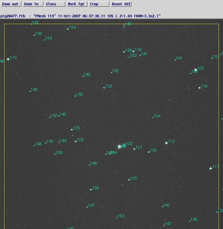
as shown in the figure in the combined image.
4. Use mklog (Linux) to get a one-line summary of all images. By using the
‘>’ symbol, the output can be redirected to a file (mklog > mylist.lis). Print
this list for future reference (lpr mylist.lis). The output will show up in room
707 (printer monet).
5. Take a first look at the images using the program camera (type camera
*.fts). The images need to be aligned so that the stars have fixed positions
on all images. To do this, use the Talon1 program crop. The command
crop –c *.fts will crop all images to the largest common area. It replaces
the original images with the cropped versions, so it cannot be undone
(except by copying images from Student Images folder again ).
6. Rerun camera. Load the
(chronologically) first image.
Choose the ‘Movie Loop’ tool
under Tools (the first image
should load). Load the second
image. Choose ‘Add’ in the
movie tool. Choose ‘Run’ in the
movie tool. This will blink the
aligned images, making the
moving asteroid obvious.
Continue to load a third, fourth,
etc image, and add them to the
movie tool, making a nice
animation of the asteroid.
7. Load the first image again. Now
that you know which object is
asteroid 4451, you need to
determine its celestial
coordinates (needed for the
automated photometry which follows). To do this, use the magnifier tool
(Click ‘Glass’). Select ‘snap to max’, ‘show 1-d plots’, and ‘overlay
gaussian fit’. Select the asteroid by clicking on it with the left mouse
button. The celestial coordinates will be displayed in green in the upper
right corner of top plot. Be sure you identify the asteroid, not a star!
8. Doing differential photometry by hand on a large number of images is
tedious and time-consuming. Fortunately, there is a program, photom,
which will automate this procedure. This program performs differential
photometry2 on all of the images, comparing the variable and check stars
1[1]
Talon (formally OCAAS) is a suite of astronomy programs written by Elwood Downey for telescope
control and image analysis. All programs are documented in the Talon manual, available in the
laboratory bookshelf.
2
Differential photometry is done by first making a circle around a star (or asteroid or other (small) bright object) and
adding up all of the ADU counts within that circle. The sky background brightness is subtracted from this total, and
the resulting ADU counts are set equal to a magnitude (in this case zero). The magnitudes of other stars in the field are
determined relative to this star by comparing ADU counts. Full documentation on photom is in the Talon manual.Astronomical Laboratory 29:137 Fall 2007
to a calibrator star, whose magnitude is arbitrarily set to zero. The input to
photom is a single text file which is easy to generate – see the Talon
manual for details. Here’s a sample input file to photom (coordinates are
made up):
55
files:
aej32101.fts
aej32102.fts
aej32103.fts
…
fixed:
04:56:23.22 +06:23:12
04:55:24:51 +06:23:45
04:55:05.05 +06:25:01
wanderer: aej32101.fts 04:56:07.23 +06:21:01 aej32132.fts 04:57.12 +06:22:45
9. The command to run photom looks like this: photom input.phot > output.lis,
where input.phot is the input file (as above), and output.lis is the output file.
D. Light Curve Generation and Period Determination
1. After running photom, the resulting output text file can be quickly plotted using
LoggerPro (You may need to strip out excess information from the file first).
Make a plot of your target (variable) star's magnitude versus Julian Date. Also
make a plot of each of your check stars versus Julian Date. All of the plots of
your check stars should be constant with time within the expected
photometric uncertainty. Be sure to include the error bars. The magnitudes of
the errors are given in the photom output file.
2. Finally, to form an estimate of the period by fitting a sine function. Find the
times of two different locations on the graphs where the light curve is
approximately the same. For example, find two peaks of the same height, and
find the times of these peaks. Subtract the smaller time from the larger time.
The resulting time is the period. (Note that the period is the time interval
between a given peak and the second peak – why?
3. You are now ready to analyze your own images. Repeat all steps in this
section on the images you obtained.You can also read