Le Digital Humanities: aspetti metodologici e pratici - Unipi
←
→
Page content transcription
If your browser does not render page correctly, please read the page content below

Dottorato di Ricerca

                            Le Digital Humanities:
                         aspetti metodologici e pratici

                         Enrica Salvatori (enrica.salvatori@unipi.it)
                          Vittore Casarosa (casarosa@isti.cnr.it)

                                     Pisa, 28 Marzo 2019

LABCD1 - 28 Marzo 2019                    DH metodologia e pratica - Enrica Salvatori e Vittore Casarosa   !1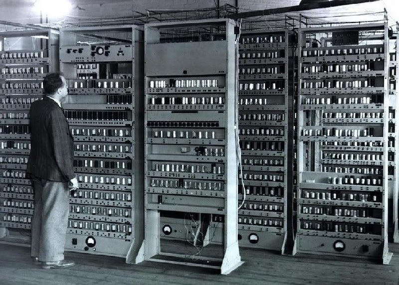
Dottorato di Ricerca

Refresher on Computer Fundamentals and
Data Representation

●       Brief History of computers
●       Architecture of a computer
●       Data representation within a computer
●       Metadata

LABCD1 - 28 Marzo 2019          DH metodologia e pratica - Enrica Salvatori e Vittore Casarosa   !2
Early visions

                                    Charles Babbage (1791-1871)
                                    Professor of Mathematics at
                                    Cambridge University (1827-1839)
                                    Difference Engine                                         1823
                                    Analytic Engine                                           1833
                                    Applications
                                    Mathematical Tables – Astronomy
                                    and Navigation
                                    Technology
                                    Jacquard’s loom (1801) and
                                    mechanical gears (steam
                                    operated)
LABCD1 - 28 Marzo 2019       DH metodologia e pratica - Enrica Salvatori e Vittore Casarosa          !3
Use of punched paper tape

LABCD1 - 28 Marzo 2019             DH metodologia e pratica - Enrica Salvatori e Vittore Casarosa   !4
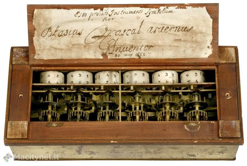
Pascaline (~ 1650)

                                                        Mechanical calculator
                                                        invented by Blaise Pascal
                                                        between 1640 and 1650.

                                                        It is not a computer (in our
                                                        meaning today) as it does
                                                        not have a program

LABCD1 - 28 Marzo 2019          DH metodologia e pratica - Enrica Salvatori e Vittore Casarosa   !5
Harvard Mark I

● Built in 1944 in IBM Endicott laboratories
  – Howard Aiken – Professor of Physics at Harvard
  – Essentially mechanical but had some electro-magnetically
    controlled relays and gears
  – Weighed 5 tons and had 750,000 components
  – A synchronizing clock that beat every 0.015 seconds (66KHz)

                         Performance:
                            0.3 seconds for addition
                            6 seconds for multiplication
                            1 minute for a sine calculation

        WW-2 Effort                   Broke down once a week!

LABCD1 - 28 Marzo 2019                DH metodologia e pratica - Enrica Salvatori e Vittore Casarosa   !6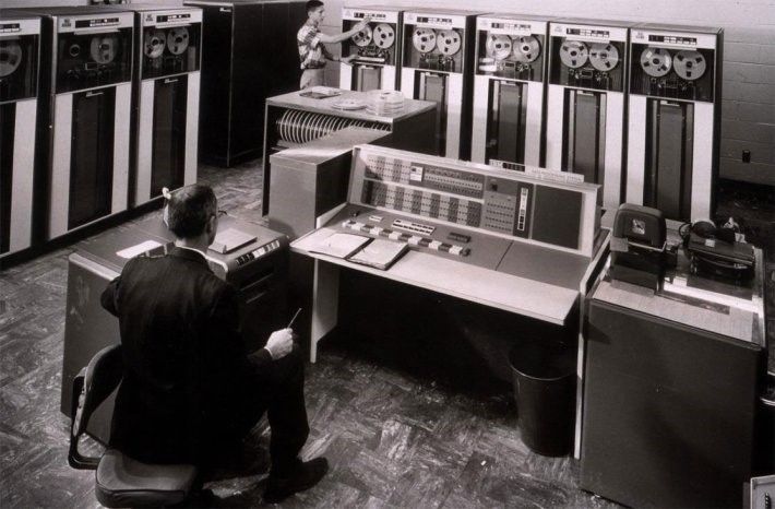
ENIAC

●       Inspired by Atanasoff and Berry, Eckert and Mauchly designed and
        built ENIAC (1943-45) at the University of Pennsylvania
●       The first, completely electronic, operational, general-purpose
        analytical calculator!
           – 30 tons, 72 square meters, 200KW
●       Performance
         – Read in 120 cards per minute
                                                                                                    WW-2 Effort
         – Addition took 200 µs, Division 6 ms
         – 1000 times faster than Mark I
●       Not very reliable!

    Application: Ballistic calculations
    angle = f (location, tail wind, cross wind,
               air density, temperature, weight of shell,
               propellant charge, ... )
LABCD1 - 28 Marzo 2019             DH metodologia e pratica - Enrica Salvatori e Vittore Casarosa                 !7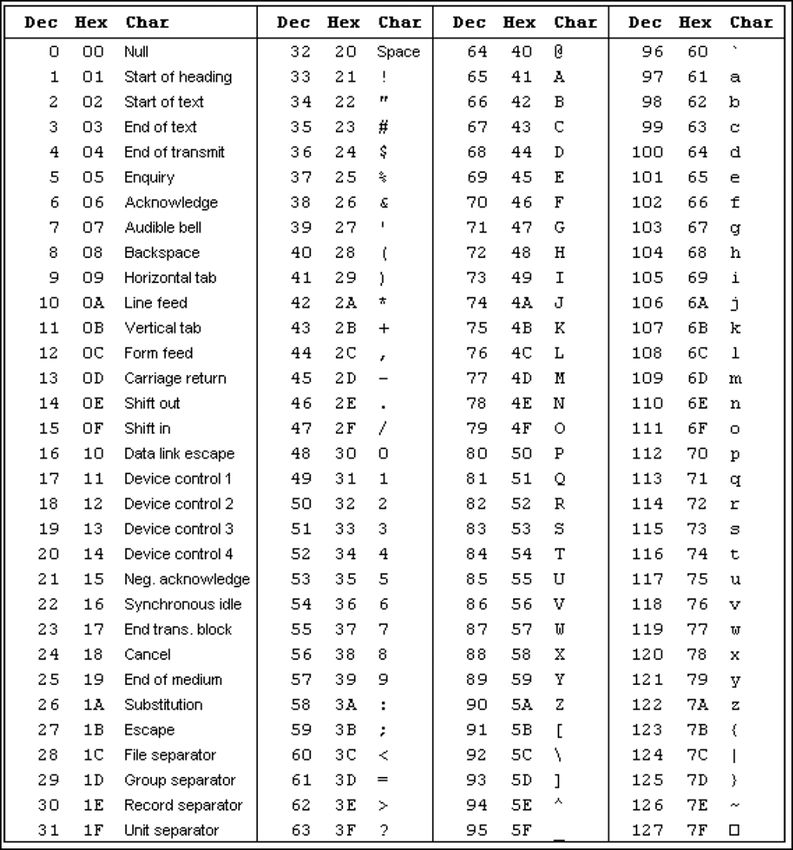
Colossus

                                                                                            Colossus (derived
                                                                                            from Mark 1 and
                                                                                            Mark 2) was used
                                                                                            in London during
                                                                                            the second World
                                                                                            War to decipher
                                                                                            secret German
                                                                                            messages (Enigma
                                                                                            machine)

LABCD1 - 28 Marzo 2019     DH metodologia e pratica - Enrica Salvatori e Vittore Casarosa                  !8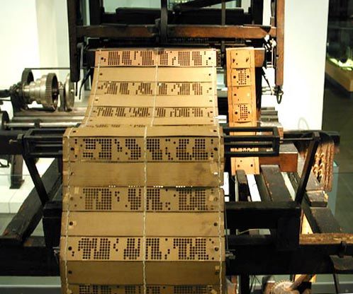
EDVAC - Electronic Discrete Variable
                               Automatic Computer

●       ENIAC’s programming system was external
           – Sequences of instructions were executed independently of the
             results of the calculation
         – Human intervention required to take instructions “out of order”
●       Eckert, Mauchly, John von Neumann and others designed EDVAC
        (1944) to solve this problem
         – Solution was the stored program computer

                             ⇒ “program can be manipulated as data”
●       First Draft of a report on EDVAC was published in 1945, but just had
        von Neumann’s signature
●       In 1973 the court of Minneapolis attributed the honor of
        inventing the computer to John Atanasoff

LABCD1 - 28 Marzo 2019                   DH metodologia e pratica - Enrica Salvatori e Vittore Casarosa   !9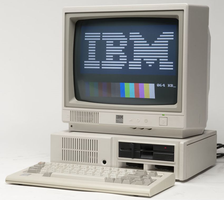
Dottorato di Ricerca

Refresher on Computer Fundamentals and
Data Representation

●       Brief History of computers
●       Architecture of a computer
●       Data representation within a computer
●       Metadata

LABCD1 - 28 Marzo 2019          DH metodologia e pratica - Enrica Salvatori e Vittore Casarosa   !10
Basic components of a computer

                                           Control Unit

                              CPU                                                                            RAM
                             Central                                                                        Random
                           Processing                                                                       Access
                              Unit                                                                          Memory

                                              I/O
                                   Input and Output Devices

LABCD1 - 28 Marzo 2019                     DH metodologia e pratica - Enrica Salvatori e Vittore Casarosa            !11
Von Neuman architecture
● The RAM contains both the program (machine instructions) and the data
● The basic model is “sequential execution”
– each instruction is extracted from memory (in sequence) and
executed
● Basic execution cycle
– Fetch instruction (from memory) at location indicated by
Location Counter
– Increment Location Counter (to point to the next instruction)
– Bring instruction to CPU
– Execute instruction
• Fetch operand from memory (if needed)
• Execute operation
• Store result
– in “registers” (temporary memory in the CPU)
– in memory (RAM)
LABCD1 - 28 Marzo 2019 DH metodologia e pratica - Enrica Salvatori e Vittore Casarosa !12Random Access Memory
● The RAM is a linear array of “cells”, usually called “words”
● The words are numbered from 0 to N, and this number is the “address” of the
word
● In order to read/write a word from/into a memory cell, the CPU has to provide
its address on the “address bus”
● A “control line” tells the memory whether it is a read or write operation
● In a read operation the memory will provide on the “data bus” the content of
the memory cell at the address provided on the “address bus”
● In a write operation the memory will store the data provided on the “data bus”
into the memory cell at the address provided on the “address bus”
LABCD1 - 28 Marzo 2019 DH metodologia e pratica - Enrica Salvatori e Vittore Casarosa !13Data within a computer
● The Control Unit, the RAM, the CPU and all the physical
components in a computer act on electrical signals and on
devices that (basically) can be in only one of two possible
states
● The two states are conventionally indicated as “zero” and
“one” (0 and 1), and usually correspond to two voltage
levels
● The consequence is that all the data within a computer (or
in order to be processed by a computer) has to be
represented with 0s and 1s, i.e. in “binary notation”
LABCD1 - 28 Marzo 2019 DH metodologia e pratica - Enrica Salvatori e Vittore Casarosa !14Basic components of a computer
Control Unit
CPU RAM
Central Random
Processing Access
Unit Memory
I/O
Input and Output Devices
LABCD1 - 28 Marzo 2019 DH metodologia e pratica - Enrica Salvatori e Vittore Casarosa !15ENIAC - Electronic Numerical Integrator
And Computer
LABCD1 - 28 Marzo 2019 DH metodologia e pratica - Enrica Salvatori e Vittore Casarosa !16EDSAC - Electronic Delay Storage
Automatic Calculator
EDSAC, University of Cambridge, UK, 1949
LABCD1 - 28 Marzo 2019 DH metodologia e pratica - Enrica Salvatori e Vittore Casarosa !17A “mainframe” in the 60’ LABCD1 - 28 Marzo 2019 DH metodologia e pratica - Enrica Salvatori e Vittore Casarosa !18
A “mainframe” in the 70’

LABCD1 - 28 Marzo 2019            DH metodologia e pratica - Enrica Salvatori e Vittore Casarosa   !19
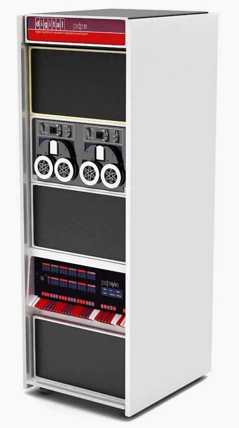
Minicomputers

LABCD1 - 28 Marzo 2019       DH metodologia e pratica - Enrica Salvatori e Vittore Casarosa   !20
Early PCs

LABCD1 - 28 Marzo 2019     DH metodologia e pratica - Enrica Salvatori e Vittore Casarosa   !21
Dottorato di Ricerca

Refresher on Computer Fundamentals and
Data Representation

●       Brief History of computers
●       Architecture of a computer
●       Data representation
●       Metadata

LABCD1 - 28 Marzo 2019          DH metodologia e pratica - Enrica Salvatori e Vittore Casarosa   !22
Representation of information
                              within a computer

●       Numbers
●       Text (characters and ideograms)
●       Documents
●       Images
●       Video
●       Audio

LABCD1 - 28 Marzo 2019               DH metodologia e pratica - Enrica Salvatori e Vittore Casarosa   !23
Positional notation base 10 Positional notation in base 10 Ten different symbols are needed for the digits (0,1,2,3,4,5,6,7,8,9) The “weight” of each digit is a power of 10 (the base) and depends on its position in the number 100=1 101=10 3 4 7 102=100 103=1000 3x10² + 4x101 + 7x100 = 347 104=10000 LABCD1 - 28 Marzo 2019 DH metodologia e pratica - Enrica Salvatori e Vittore Casarosa !24
Roman numbers

       Roman numbers are not positional
       They are the sum of the values, unless a smaller
       value precedes a larger one; in that case the
       smaller value is subtracted from the larger one

                         I=1                    XXVII = 27
                         V=5                    XXXIV = 34
                         X=10                   XLV = 45
                         L=50                   MCMXCIX = 1999
                         C=100                  MMVIII = 2008
                         D=500                  MMIX = 2009
                         M=1000                 MMX = 2010
LABCD1 - 28 Marzo 2019             DH metodologia e pratica - Enrica Salvatori e Vittore Casarosa   !25
Positional notation base 8
Positional notation in base 8
Eight different symbols are needed for the digits (0,1,2,3,4,5,6,7)
The “weight” of each digit is a power of 8 (the base) and depends
on its position in the number
80=1
81=8 3 4 7
82=64
83=512 3x82 + 4x81 + 7x80
84=4096 192 + 32 + 7 = 231
LABCD1 - 28 Marzo 2019 DH metodologia e pratica - Enrica Salvatori e Vittore Casarosa !26Positional notation base 16
Positional notation in base 16
Sixteen different symbols are needed for the digits (0,1,2,3,4,5,6,7,
8,9,A,B,C,D,E,F)
The “weight” of each digit is a power of 16 (the base) and depends
on its position in the number
160=1 3 B F
161=16
162=256 3x162 + Bx161 + Fx160
163=4096 3x256 + 11x16 + 15x1
164=65536 768 + 176 + 15 = 959
LABCD1 - 28 Marzo 2019 DH metodologia e pratica - Enrica Salvatori e Vittore Casarosa !27Positional notation base 2
Positional notation in base 2
Two different symbols are needed for the digits (0,1)
The “weight” of each digit is a power of 2 (the base) and depends
on its position in the number
20=1
21=2
22=4 1 0 1 1
23=8
24=16 1x23 + 0x22 + 1x21 + 1x20
25=32 1x8 + 0x4 + 1x2 + 1x1
26=64
8 + 0 + 2 + 1 = 11
27=128
28=256
LABCD1 - 28 Marzo 2019 DH metodologia e pratica - Enrica Salvatori e Vittore Casarosa !28Powers of 2
20=1 29=512
21=2 210=1024 1K
22=4 211=2048 2K
23=8 212=4096 4K
24=16 213=8192 8K
25=32 214=16384 16K
26=64 215=32768 32K
27=128 216=65356 64K
28=256 ......
220=1.048.576 1024K 1M
230=1.073.741.824 1024M 1G
232=4.271.406.736 4096M 4G
LABCD1 - 28 Marzo 2019 DH metodologia e pratica - Enrica Salvatori e Vittore Casarosa !29Binary and hexadecimal numbers
20=1 0000=0 1000=8
21=2 0001=1 1001=9
22=4 0010=2 1010=10 A
23=8 0011=3 1011=11 B
24=16 0100=4 1010=12 C
25=32 0101=5 1011=13 D
26=64 0110=6 1110=14 E
27=128 0111=7 1111=15 F
28=256
10000=16 10
decimal and exadecimal
decimal 01011011 si può rappresentare
hexadecimal in esadecimale come 5D
LABCD1 - 28 Marzo 2019 DH metodologia e pratica - Enrica Salvatori e Vittore Casarosa !30Size of digital information
1 GB = 1000 MB
1 TB = 1000 GB
1 PB = 1000 TB
1 EB = un milione TB
1 ZB = un miliardo TB
The digital content in
the world in 2018 was
estimated to be about
35 zettabytes
LABCD1 - 28 Marzo 2019 DH metodologia e pratica - Enrica Salvatori e Vittore Casarosa !31Representation of information
within a computer
● Numbers
● Text (characters and ideograms)
● Documents
● Images
● Video
● Audio
LABCD1 - 28 Marzo 2019 DH metodologia e pratica - Enrica Salvatori e Vittore Casarosa !32Representation of characters
● The “natural” way to represent (alphanumeric)
characters (and symbols) within a computer is to
associate a character with a number, defining a
“coding table”
● How many bits are needed to represent the Latin
alphabet ?
LABCD1 - 28 Marzo 2019 DH metodologia e pratica - Enrica Salvatori e Vittore Casarosa !33The ASCII characters
The 95
printable
ASCII
characters,
numbered
from 32 to 126
(decimal)
33 control
characters
LABCD1 - 28 Marzo 2019 DH metodologia e pratica - Enrica Salvatori e Vittore Casarosa !34ASCII table (7 bits) LABCD1 - 28 Marzo 2019 DH metodologia e pratica - Enrica Salvatori e Vittore Casarosa !35
Representation standards
●       ASCII 7 bits (late fifties)
         – American Standard Code for Information Interchange
         – 7 bits for 128 characters (Latin alphabet, numbers, punctuation, control
           characters)
●       EBCDIC (early sixties)
           – Extended Binary Code Decimal Interchange Code
         – 8 bits; defined by IBM in early sixties, still used and supported on many
           computers
●       ASCII 8 bits (ISO 8859-xx) extends original ASCII to 8 bits to include
        accented letters and non Latin alphabets (e.g. Greek, Russian)
●       UNICODE or ISO-10646 (1993)
         – Merged efforts of the Unicode Consortium and ISO
         – UNIversal CODE still evolving
         – It incorporates all(?) the pre-existing representation standards
         – Basic rule: round trip compatibility
                         • Side effect is multiple representations for the same character

LABCD1 - 28 Marzo 2019                                  DH metodologia e pratica - Enrica Salvatori e Vittore Casarosa   !36
ISO-8859-xx (ASCII 8-bits)
● Developed by ISO (International Organization for
Standardization)
● There are 16 different tables coding characters
with 8 bit
● Each table includes ASCII (7 bits) in the lower part
and other characters in the upper part for a total of
191 characters and 32 control codes
● It is also known as ISO-Latin–xx (includes all the
characters of the “Latin alphabet”)
LABCD1 - 28 Marzo 2019 DH metodologia e pratica - Enrica Salvatori e Vittore Casarosa !37ISO-8859-xx code pages ● 8859-1 Latin-1 Western European languages ● 8859-2 Latin-2 Central European languages ● 8859-3 Latin-3 South European languages ● 8859-4 Latin-4 North European languages ● 8859-5 Latin/Cyrillic Slavic languages ● 8859-6 Latin/Arabic Arabic language ● 8859-7 Latin/Greek modern Greek alphabet ● 8859-8 Latin/Hebrew modern Hebrew alphabet ● 8859-9 Latin-5 Turkish language (similar to 8859-1) ● 8859-10 Latin-6 Nordic languages (rearrangement of Latin-4) ● 8859-11 Latin/Thai Thai language ● 8859-12 Latin/Devanagari Devanagari language (abandoned in 1997) ● 8859-13 Latin-7 Baltic Rim languages ● 8859-14 Latin-8 Celtic languages ● 8859-15 Latin-9 Revision of 8859-1 ● 8859-16 Latin-10 South-Eastern European languages LABCD1 - 28 Marzo 2019 DH metodologia e pratica - Enrica Salvatori e Vittore Casarosa !38
Representation standards

●       ASCII (late fifties)
         – American Standard Code for Information Interchange
         – 7 bits for 128 characters (Latin alphabet, numbers, punctuation, control
           characters)
●       EBCDIC (early sixties)
           – Extended Binary Code Decimal Interchange Code
         – 8 bits; defined by IBM in early sixties, still used and supported on many
           computers
●       ISO 8859-1 extends ASCII to 8 bits (accented letters, non Latin characters)
●       UNICODE or ISO-10646 (1993)
         – Merged efforts of the Unicode Consortium and ISO
         – UNIversal CODE still evolving
         – It incorporates all(?) the pre-existing representation standards
         – Basic rule: round trip compatibility
                         • Side effect is multiple representations for the same character

LABCD1 - 28 Marzo 2019                                  DH metodologia e pratica - Enrica Salvatori e Vittore Casarosa   !39
UNICODE
● In Unicode, the word “character” refers to the notion of the abstract
form of a “letter”, in a very broad sense
– a letter of an alphabet
– a mark on a page
– a symbol (in a language)
● A “glyph” is a particular rendition of a character (or composite
character). The same Unicode character can be rendered by many
glyphs
– Character “a” in 12-point Helvetica, or
– Character “a” in 16-point Times
● In Unicode each “character” has a name and a numeric value (called
“code point”), indicated by U+hex value.
For example, the letter “G” has:
– Unicode name: “LATIN CAPITAL LETTER G”
– Unicode value: U+0047 (see ASCII codes)
LABCD1 - 28 Marzo 2019 DH metodologia e pratica - Enrica Salvatori e Vittore Casarosa !40Unicode representation
● The Unicode standard has specified (and assigned values
to) about 96.000 characters
● Representing Unicode characters (code points)
– 32 bits in ISO-10646
– 21 bits in the Unicode Consortium
● In the 21 bit address space, there are 32 “planes” of 64K
characters each (256X256)
● Only 6 planes defined as of today, of which only 4 are
actually “filled”
● Plane 0, the Basic Multingual Plane, contains most of the
characters used (as of today) by most of the languages
used in the Web
LABCD1 - 28 Marzo 2019 DH metodologia e pratica - Enrica Salvatori e Vittore Casarosa !41The planes of Unicode
256 characters (8 bits)
In each row
hex hex
00 FF
00
256 characters (8 bits)
In each column
64K characters
In each plane FF
LABCD1 - 28 Marzo 2019 DH metodologia e pratica - Enrica Salvatori e Vittore Casarosa !42Unicode planes
Plane 0 Basic Multilingual U+0000 to modern languages and special
Plane U+FFFF characters. Includes a large number of
Chinese, Japanese and Korean (CJK)
characters.
Plane 1 Supplementary U+10000 to historic scripts and musical and
Multilingual Plane U+1FFFF mathematical symbols
Plane 2 Supplementary U+20000 to rare Chinese characters
Ideographic Plane U+2FFFF
Plane Supplementary U+E0000 to non-recommended language tag and
14 Special-purpose U+EFFFF variation selection characters
Plane
Plane Supplementary U+F0000 to private use (no character is specified)
15 Private Use Area- U+FFFFF
A
Plane Supplementary U+100000 private use (no character is specified)
16 Private Use Area- to
B U+10FFFF
LABCD1 - 28 Marzo 2019 DH metodologia e pratica - Enrica Salvatori e Vittore Casarosa !43Unicode charts
Language characters Kannada Language specific characters Numbers
(Chinese, Japanese, Korean)
Basic Latin Khmer Symbols Bopomofo Extended Aegean Numbers
Latin-1 Supplement Khmer Bopomofo Number Forms
CJK Compatibility Forms
Latin Extended-A Lao CJK Compatibility Ideographs Other symbols
Latin Extended-B Limbu Supplement
Latin Extended Additional Linear B Ideograms CJK Compatibility Ideographs Braille Patterns
CJK Compatibility Byzantine Musical Symbols
Linear B Syllabary CJK Radicals Supplement Combining Diacritical Marks for
Language specific Malayalam Symbols
CJK Symbols and Punctuation Control Pictures
characters CJK Unified Ideographs Extension A Currency Symbols
Alphabetic Presentation Forms Mongolian CJK Unified Ideographs Extension B Enclosed Alphanumerics
Arabic Presentation Forms-A Myanmar CJK Unified Ideographs Letterlike Symbols
Enclosed CJK Letters and Months Miscellaneous Technical
Arabic Presentation Forms-B Ogham Hangul Compatibility Jamo Musical Symbols
Arabic Old Italic Hangul Jamo Optical Character Recognition
Armenian Oriya Hangul Syllables Tai Xuan Jing Symbols
Hiragana Yijing Hexagram Symbols
Bengali Osmanya Ideographic Description Characters
Buhid Runic Kanbun Character modifiers and punctuation
Kangxi Radicals Combining Diacritical Marks
Cherokee Shavian Katakana Phonetic Extensions IPA Extensions
Cypriot Syllabary Sinhala Katakana Phonetic Extensions
Cyrillic Supplement Syriac Spacing Modifier Letters
Graphic symbols Combining Half Marks
Cyrillic Tagalog Arrows General Punctuation
Deseret Tagbanwa Block Elements Superscripts and Subscripts
Box Drawing
Devanagari Tai Le Geometric Shapes Miscellaneous
Ethiopic Tamil Misc. Symbols and Arrows Halfwidth and Fullwidth Forms
Georgian Telugu Supplemental Arrows-A High Private Use Surrogates
Supplemental Arrows-B High Surrogates
Gothic Thaana Low Surrogates
Greek and Coptic Thai Pictorial symbols Private Use Area
Greek Extended Tibetan Dingbats Small Form Variants
Miscellaneous Symbols Specials
Gujarati Ugaritic Supplementary Private Use Area-A
Gurmukhi Unified Canadian Aboriginal Mathematical symbols Supplementary Private Use Area-B
Math. Alphanumeric Symbols Tags
Syllabics Math. Operators Variation Selectors Supplement
Hanunoo Yi Radicals Miscellaneous Math. Symbols-A Variation Selectors
Hebrew Yi Syllables Miscellaneous Math. Symbols-B
Supplemental Math. Operators
LABCD1 - 28 Marzo 2019 DH metodologia e pratica - Enrica Salvatori e Vittore Casarosa !44Beginning of BMP
in this table each “column” represents 16 characters
LABCD1 - 28 Marzo 2019 DH metodologia e pratica - Enrica Salvatori e Vittore Casarosa !45Unicode encoding
● UTF-32 (fixed length, four bytes)
– UTF stands for “UCS Transformation Format” (UCS stands for “Unicode
Character Set”)
– UTF-32BE and UTF-32LE have a “byte order mark” to indicate
“endianness”
● UTF-16 (variable length, two bytes or four bytes)
– All characters in the BMP represented by two bytes
– The 21 bits of the characters outside of the BMP are divided in two parts
of 11 and 10 bits; to each part is added an offset to bring it in the
“surrogate zone” of the BMP (low surrogate at D800 and high surrogate at
DC800)
– in other words, they are represented as two characters in the BMP
– UTF-16BE and UTF-16LE to indicate “endianness”
● UTF-8 (variable length, most often one byte)
– Characters in the 7-bit ASCII represented by one byte
– Variable length encoding (2, 3 or 4 bytes) for all other characters
LABCD1 - 28 Marzo 2019 DH metodologia e pratica - Enrica Salvatori e Vittore Casarosa !46Unicode example
First four characters of Welcome
LABCD1 - 28 Marzo 2019 DH metodologia e pratica - Enrica Salvatori e Vittore Casarosa !47UTF-8 LABCD1 - 28 Marzo 2019 DH metodologia e pratica - Enrica Salvatori e Vittore Casarosa !48
Representation of information
                              within a computer

●       Numbers
●       Text (characters and ideograms)
●       Documents
●       Images
●       Video
●       Audio

LABCD1 - 28 Marzo 2019               DH metodologia e pratica - Enrica Salvatori e Vittore Casarosa   !49
The editors ● Text processing applications started already in the early days of the computers (sixties) ● A “text processor” (or editor) has two main functions: – processing the text (delete, replace, insert, etc.) – specifying the format (bold, center, new line, etc.) ● The first editors were using a “mark up” language (i.e. commands intermixed with the text) to provide formatting instructions (only limited interactivity available through typewriter-like terminals) ● The “second generation” editors were using the WYSIWYG paradigm: What You See Is What You Get (much better interactivity available with display and mouse) LABCD1 - 28 Marzo 2019 DH metodologia e pratica - Enrica Salvatori e Vittore Casarosa !50
Representing documents

●       Plain text
           – No information about structure
           – Different representation for line breaks
                         • Windows represent a new line with the sequence “carriage return” followed by
                           “line feed”
                         • Unix and Apple/Mac represent a new line with “line feed” only
●       Page description languages
           – PostScript
           – PDF – Portable Document Format
●       Word processors
           – RTF – Rich Text Format
           – Microsoft Word
           – LaTeX

LABCD1 - 28 Marzo 2019                               DH metodologia e pratica - Enrica Salvatori e Vittore Casarosa   !51
PostScript
● First commercially available page description language (Adobe 1985)
● It is a real programming language (variables, procedures, etc.) and a
PostScript document is actually a “PostScript program”
● A page description comprises a number of graphical drawing instructions,
including those that draw letters in a specific font in a specific size
– Type-1 (Adobe) fonts versus TrueType (Apple)
● The document can be printed (or displayed) by having a “PostScript
interpreter” executing the program
● The “abstract” PostScript description is converted to a matrix of dots
(“rasterization” or “rendering”)
● PostScript initially designed for printing
– Photo typesetters resolution up to 12000 dpi (dots per inch)
● PostScripts documents in a Digital Library
– Extraction of text not always immediate
– Digital Library must have a PostScript interpreter
LABCD1 - 28 Marzo 2019 DH metodologia e pratica - Enrica Salvatori e Vittore Casarosa !52PDF
Portable Document Format
● Successor to PostScript, to include good support for
displays
● No longer a real programming language
● It defines an overall structure for a pdf document
– Header, objects, cross-references, trailer
● Support for interactive display
– Hierarchically structured content
– Random access to pages
– Navigation within a document
– Support of hyperlinks
– Support of “searchable images”
– Limited editing capabilities
LABCD1 - 28 Marzo 2019 DH metodologia e pratica - Enrica Salvatori e Vittore Casarosa !53RTF – Rich Text Format
● Dates back to 1987
● Designed primarily to exchange documents among
different word processors
● Description must allow a word processor to change
“everything” (fonts, typesetting, tables, graphics, etc.)
● It defines an overall structure for a rtf document
– Header, body
LABCD1 - 28 Marzo 2019 DH metodologia e pratica - Enrica Salvatori e Vittore Casarosa !54LaTeX
● Widely used in the scientific and mathematical communities
● Based on TeX, defined in the late seventies by Don Knuth, to overcome the
limitations of the typesetters available at the time
● LaTeX documents are expressed in plain text, to expose all the details of the
internal representation
– Any text editor on any platform can be used to compose LaTeX document
– Converted to a page description language (typically PostScript or PDF) to
get the formatted document
● Simple document structure
– Preamble to set the defaults and the global features
– Structured (sections and subsections) document content
● Highly customizable with “external packages”
● Text extraction not so immediate
– A single document may occupy several files
– Possibility of “too much” customization
LABCD1 - 28 Marzo 2019 DH metodologia e pratica - Enrica Salvatori e Vittore Casarosa !55Representation of information
within a computer
● Numbers
● Text (characters and ideograms)
● Documents
● Images
● Video
● Audio
LABCD1 - 28 Marzo 2019 DH metodologia e pratica - Enrica Salvatori e Vittore Casarosa !56Welcome
Welcome to image
representation and
compression
LABCD1 - 28 Marzo 2019 DH metodologia e pratica - Enrica Salvatori e Vittore Casarosa !57Representation of images
● Vector formats (geometric description)
– Postscript
– PDF
– SVG (Scalable Vector Graphics)
– SWF (ShockWave Flash)
• from FutureWave Software to Macromedia to Adobe
• vector-based images, plus audio, video and interactivity
• can be played by Adobe Flash Player (browser plug-in or
stand-alone)
● Raster formats (array of “picture elements”, called “pixels”)
LABCD1 - 28 Marzo 2019 DH metodologia e pratica - Enrica Salvatori e Vittore Casarosa !58Picture elements (pixels)
A pixel must be
small enough so
that its color can
be considered
uniform for the
whole pixel.
Inside the
computer, a pixel is
represented with a
number
representing its
color.
LABCD1 - 28 Marzo 2019 DH metodologia e pratica - Enrica Salvatori e Vittore Casarosa !59Raster format
● In raster format an image (picture) is represented by a matrix of
“pixels”
● Colors are represented by three numbers, one for each “color
component”
● The quality of a picture is determined by:
– The number of rows and columns in the matrix
• Very often it is expressed as “dots per inch” (dpi)
• 200-4800 dpi (most common ranges)
– The number of bits representing one pixel (called depth)
• 1 bit for black and white
• 8-16 bits for gray scale (most common ranges)
• 12-48 bits for color images (most common ranges)
● Big file sizes for (uncompressed color) pictures
– For example, one color page scanned at 600 dpi is about 100 MB
LABCD1 - 28 Marzo 2019 DH metodologia e pratica - Enrica Salvatori e Vittore Casarosa !60RGB and CMY color components
Additive color mixing Subtractive color mixing
LABCD1 - 28 Marzo 2019 DH metodologia e pratica - Enrica Salvatori e Vittore Casarosa !61Common raster
image file formats
● Big file sizes for (uncompressed color) pictures.
Compression is (usually) needed
● Lossless compression
– G3, G4, JBIG
– GIF, PNG
● Lossy compression
– JPEG
● Image containers
– TIFF
● BMP, RAW (sensor output), DNG (Digital
Negative), etc.
LABCD1 - 28 Marzo 2019 DH metodologia e pratica - Enrica Salvatori e Vittore Casarosa !62Compression process
String of symbols out of a
given alphabet
uncompressed string
encoder
network,
storage, ...
uncompressed string compressed string
decoder
LABCD1 - 28 Marzo 2019 DH metodologia e pratica - Enrica Salvatori e Vittore Casarosa !63Lossless data compression
● The idea of text compression, or more generally data compression, is
that when the data is not needed for processing (e.g. when in transit
over a network or when stored on secondary storage), then it can be
represented in a more compact form (with less bits), provided that it
can be brought back to the original format when needed, i.e. we want
to make a “lossless compression”.
● Given a string of symbols of a given alphabet (e.g. a string of
characters out of the 26 letters of the English alphabet, or a string of
numbers out of the 10 digits), which is represented in the computer by
N bits, the compression process takes this string and represents it in a
different way so that after compression the string takes n bits, with
nCommon raster
image file formats
● Lossless compression
– G3, G4, JBIG
– GIF, PNG
● Lossy compression
– JPEG
● Image containers
– TIFF
● BMP, RAW (sensor output), DNG (Digital
Negative), etc.
LABCD1 - 28 Marzo 2019 DH metodologia e pratica - Enrica Salvatori e Vittore Casarosa !65Lossless compression: G3, G4, JBIG
● CCITT standard (since late seventies) for fax
– Comite’ Consultatif Internationale de Telegraphie et de Telephonie,
part of ITU – International Telecommunications Union
● Specifies resolution
– 200 x 100 dpi (standard) or 200 x 200 dpi (hig resolution)
● Basically bi-level documents (black and white), even if G4 includes also
provisions for optional greyscale and color images
● A one-page A4 document contains 1728x1188 pixels (bits), which is about
2 MB of data (too much to be sent over telephone lines, especially at that
time)
● G3 specifies two coding (compression) methods.
– One-dimensional (each line treated separately)
– Two-dimensional (called READ, exploits coherence between
succesive scan lines)
● G4 and JBIG are more recent versions of the standard, which allow a
much better compression
LABCD1 - 28 Marzo 2019 DH metodologia e pratica - Enrica Salvatori e Vittore Casarosa !66Common raster
image file formats
● Lossless compression
– G3, G4, JBIG
– GIF, PNG
● Lossy compression
– JPEG
● Image containers
– TIFF
● BMP, RAW (sensor output), DNG (Digital
Negative), etc.
LABCD1 - 28 Marzo 2019 DH metodologia e pratica - Enrica Salvatori e Vittore Casarosa !67Pixel representation in GIF
color table
24-36-48 bits
image - 8 bits/pixel
0
sequence of rows
0
......
pointer to
...... color table ......
. .
N 255
LABCD1 - 28 Marzo 2019 DH metodologia e pratica - Enrica Salvatori e Vittore Casarosa !68GIF format LABCD1 - 28 Marzo 2019 DH metodologia e pratica - Enrica Salvatori e Vittore Casarosa !69
GIF and PNG
●       GIF – Graphics Interchage Format, is probably the most used “lossless”
        compression format for images (late eighties)
●       Each file may contain several images (it supports animation)
●       In an image, each pixel is represented by 8 bits (or less), and the value is an
        index in a color table, which can be included in the file (if not included, a
        standard color table is used)
●       The color table has 256 entries, therefore a GIF image can have a “palette” of
        at most 256 colors (which is much less than the colors actually in the picture)
●       The pixel index values are compressed using the LZW method
●       The LZW coded information is divided in blocks, preceded by a header with a
        byte count, so it is possible to skip over images without decompressing them
●       PNG (Portable Network Graphics) is essentially the same, and was defined
        some years later to avoid the use of the “proprietary” LZW compression
        algorithm
         – PNG uses “public domain” gzip or deflate methods
         – It incorporates also several improvements over GIF

LABCD1 - 28 Marzo 2019                 DH metodologia e pratica - Enrica Salvatori e Vittore Casarosa   !70
Common raster
image file formats
● Lossless compression
– G3, G4, JBIG
– GIF, PNG
● Lossy compression
– JPEG
● Image containers
– TIFF
● BMP, RAW (sensor output), DNG (Digital
Negative), etc.
LABCD1 - 28 Marzo 2019 DH metodologia e pratica - Enrica Salvatori e Vittore Casarosa !71JPEG
● For grayscale and color images, lossless compression still results in
“too many bits”
● Lossy compression methods take advantage from the fact that the
human eye is less sensitive to small greyscale or color variation in an
image
● JPEG - Joint Photographic Experts Group and Joint Binary Image
Group, part of CCITT and ISO
● JPEG can compress down to about one bit per pixel (starting with 8-48
bits per pixel) still having excellent image quality
– Not very good for fax-like images
– Not very good for sharp edges and sharp changes in color
● The encoding and decoding process is done on an 8x8 block of pixels
(separately for each color component)
LABCD1 - 28 Marzo 2019 DH metodologia e pratica - Enrica Salvatori e Vittore Casarosa !72JPEG encoding and decoding LABCD1 - 28 Marzo 2019 DH metodologia e pratica - Enrica Salvatori e Vittore Casarosa !73
JPEG – Final comments

●       Arithmetic coding instead of Huffman coding (10% improvement in
        compression)
●       JPEG-2000 - Use of wavelets instead of DCT (20% improvement in
        compression, better quality for images with sharp edges)
●       JPEG-LS – state of the art lossless compression
           – For each pixel, what is coded is the difference between the actual pixel
             value and a prediction of pixel value based on the pixel context
●       Compression rates
           – 0.25–0.5 bit/pixel: moderate to good quality, sufficient for some
             applications
           – 0.5–0.75 bit/pixel: good to very good quality, sufficient for many
             applications
           – 0.75–1.5 bit/pixel: excellent quality, sufficient for most applications
           – 1.5–2 bits/pixel: usually indistinguishable from the original, sufficient for
             the most demanding applications

LABCD1 - 28 Marzo 2019                     DH metodologia e pratica - Enrica Salvatori e Vittore Casarosa   !74
Common raster
image file formats
● Lossless compression
– G3, G4, JBIG
– GIF, PNG
● Lossy compression
– JPEG
● Image containers
– TIFF
● BMP, RAW (sensor output), DNG (Digital
Negative), etc.
LABCD1 - 28 Marzo 2019 DH metodologia e pratica - Enrica Salvatori e Vittore Casarosa !75TIFF
● Tagged Image File Format – file format that includes
extensive facilities for descriptive metadata
– note that TIFF tags are not the same thing as XML tags
● Owned by Adobe, but public domain (no licensing)
● Large number of options
– Problems of backward compatibility
– Problems of interoperability
(Thousands of Incompatible File Formats )
● Can include (and describe) four types of images
– bilevel (black and white), greyscale, palette-color, full-color
● Support of different color spaces
● Support of different compression methods
● Much used in digital libraries and archiving
LABCD1 - 28 Marzo 2019 DH metodologia e pratica - Enrica Salvatori e Vittore Casarosa !76Common raster
image file formats
● Lossless compression
– G3, G4, JBIG
– GIF, PNG
● Lossy compression
– JPEG
● Image containers
– TIFF
● BMP, RAW (sensor output), DNG (Digital
Negative), etc.
LABCD1 - 28 Marzo 2019 DH metodologia e pratica - Enrica Salvatori e Vittore Casarosa !77Representation of information
within a computer
● Numbers
● Text (characters and ideograms)
● Documents
● Images
● Video
● Audio
LABCD1 - 28 Marzo 2019 DH metodologia e pratica - Enrica Salvatori e Vittore Casarosa !78Representing video
● Sequence of frames (still images) displayed with a given
frequency
– NTSC 30 f/s, PAL 25 f/s, HDTV 60 f/s
● Resolution of each frame depend on quality and video
standard
– 720x480 NTSC, 768x576 PAL, 1920x1080 HDTV, 3840×2160
UltraHD, 4096×2160 4K
● Uncompressed video requires “lots of bits”
– e.g. 1920x1080x24x30 = ~ 1,5 GB/sec
● It is possible to obtain very high compression rates
– Spatial redundancy (within each frame, JPEG-like)
– Temporal redundancy (across frames)
LABCD1 - 28 Marzo 2019 DH metodologia e pratica - Enrica Salvatori e Vittore Casarosa !79MPEG
● MPEG - Motion Picture Experts Group established in 1988
as a committee of ISO to develop an open standard for
digital TV format (CD-ROM)
● Business motivations
– Two types of application for videos:
• Asymmetric (encoded once, decoded many times)
– Broadcasting, CD’s
– Video games, Video on Demand
• Symmetric (encoded once, decoded once)
– Video phone, video mail …
● Design point for MPEG-1
– Video at about 1.5 Mbits/sec
– Audio at about 64-192 kbits/channel
LABCD1 - 28 Marzo 2019 DH metodologia e pratica - Enrica Salvatori e Vittore Casarosa !80Spatial Redundancy Reduction (DCT)
“Intra-Frame
Encoded”
Quantization Zig-Zag Scan,
• major reduction
• controls ‘quality’ Run-length
coding
LABCD1 - 28 Marzo 2019 DH metodologia e pratica - Enrica Salvatori e Vittore Casarosa !81Temporal Redundancy Reduction (motion
vectors)
LABCD1 - 28 Marzo 2019 DH metodologia e pratica - Enrica Salvatori e Vittore Casarosa !82Types of frames in compression
● MPEG uses three types of frames for video coding
(compressing)
– I frames: intra-frame coding
• Coded without reference to other frames
• Moderate compression (DCT, JPEG-like)
• Access points for random access
– P frames: predictive-coded frames
• Coded with reference to previous I or P frames
– B frames: bi-directionally predictive coded
• Coded with reference to previous and future I and P frames
• Highest compression rates
LABCD1 - 28 Marzo 2019 DH metodologia e pratica - Enrica Salvatori e Vittore Casarosa !83Temporal Redundancy Reduction
● I frames are independently encoded
● P frames are based on previous I and P frames
● B frames are based on previous and following I and P
frames
LABCD1 - 28 Marzo 2019 DH metodologia e pratica - Enrica Salvatori e Vittore Casarosa !84Sequence of frames LABCD1 - 28 Marzo 2019 DH metodologia e pratica - Enrica Salvatori e Vittore Casarosa !85
Typical Compression Performance

                          Type Size Compression
                          ---------------------
                             I    18 KB    7:1
                             P     6 KB   20:1
                             B   2.5 KB   50:1
                            Avg 4.8 KB    27:1
                          ---------------------

LABCD1 - 28 Marzo 2019            DH metodologia e pratica - Enrica Salvatori e Vittore Casarosa   !86
Representation of information
within a computer
● Numbers
● Text (characters and ideograms)
● Documents
● Images
● Video
● Audio
LABCD1 - 28 Marzo 2019 DH metodologia e pratica - Enrica Salvatori e Vittore Casarosa !87Digitization of audio (analog) signals
• sampling rate should be at least the double of the highest
frequency in the signal (Shannn theorem)
•8-16 bit per sample
LABCD1 - 28 Marzo 2019 DH metodologia e pratica - Enrica Salvatori e Vittore Casarosa !88Representing audio
● MPEG-1 defines three different schemes (called layers) for
compressing audio
● All layers support sampling rates of 32, 44.1 and 48 kHz
● MP3 is MPEG-1 Layer 3
LABCD1 - 28 Marzo 2019 DH metodologia e pratica - Enrica Salvatori e Vittore Casarosa !89MPEG summary
● The main aim of MPEG-1 and –2 is to efficiently code compressed
video and audio (e.g. MP3 in MPEG-1 and DVD video in MPEG-2)
● The main aim of MPEG-4 is to extend the audio/video stream with
additional information and capabilities, such as still images, 3D
objects, animation (a la GIF), some interactivity, etc. It contains also
further improvements for compression (used in DivX)
● MPEG-1, -2 and –4 have been defined to represent, in a compressed
form, the multimedia content (“the bits”)
● MPEG-7 has been defined with a different aim, i.e. to represent
information about the multimedia content (it is the “bits about the bits”)
and is substantially a metadata set
● MPEG-21 has been defined with the aim of providing a further level of
description of the multimedia content, to represent its complete life-
cycle and to represent it in a more abstract way, as “Digital Item”
LABCD1 - 28 Marzo 2019 DH metodologia e pratica - Enrica Salvatori e Vittore Casarosa !90Multimedia file formats
● A muxer (abbreviation of multiplexer) is a “container” file
that can contain several video and audio streams,
compressed with codecs
– Common file formats are AVI, DIVx, FLV, MKV, MOV,
MP4, OGG, VOB, WMV, 3GPP
● A codec (abbreviation of coder/decoder) is a “system” (a
series of algorithms) to compress video and audio streams
– Common video codecs are HuffyYUV, FLV1, HEVC,
Mpeg2, xvid4, x264, H264, H265
– Common audio codecs are AAC, AC3, MP3, PCM,
Vorbis
LABCD1 - 28 Marzo 2019 DH metodologia e pratica - Enrica Salvatori e Vittore Casarosa !91Dottorato di Ricerca Refresher on Computer Fundamentals and Data Representation ● Brief History of computers ● Architecture of a computer ● Data representation ● Metadata LABCD1 - 28 Marzo 2019 DH metodologia e pratica - Enrica Salvatori e Vittore Casarosa !92
You can also read