Computational Astrophysics I - Introduction and Basic Concepts - Helge Todt April 21, 2020
←
→
Page content transcription
If your browser does not render page correctly, please read the page content below
Computational Astrophysics I –
Introduction and Basic Concepts

            Helge Todt

           April 21, 2020
Contents
1 Introduction, Unix, C++                                                                                                                5
  1.1 Introduction . . . . . . . . . . . . .    .   .   .   .   .   .   .   .   .   .   .   .   .   .   .   .   .   .   .   .   .   .    5
  1.2 About computers . . . . . . . . . .       .   .   .   .   .   .   .   .   .   .   .   .   .   .   .   .   .   .   .   .   .   .    7
       1.2.1 Components of a computer           .   .   .   .   .   .   .   .   .   .   .   .   .   .   .   .   .   .   .   .   .   .    9
  1.3 The stud domain and cluster . . .         .   .   .   .   .   .   .   .   .   .   .   .   .   .   .   .   .   .   .   .   .   .   12
       1.3.1 The computer lab . . . . . .       .   .   .   .   .   .   .   .   .   .   .   .   .   .   .   .   .   .   .   .   .   .   12
       1.3.2 Linux . . . . . . . . . . . .      .   .   .   .   .   .   .   .   .   .   .   .   .   .   .   .   .   .   .   .   .   .   13
  1.4 Shell and shell . . . . . . . . . . . .   .   .   .   .   .   .   .   .   .   .   .   .   .   .   .   .   .   .   .   .   .   .   15
       1.4.1 Directories . . . . . . . . .      .   .   .   .   .   .   .   .   .   .   .   .   .   .   .   .   .   .   .   .   .   .   16

                                                                                                                                        3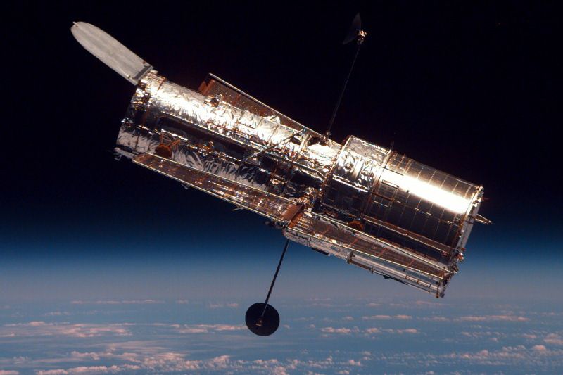
1 Introduction, Unix, C++

1.1 Introduction
Conventions of used fonts
In Tab. 1.1 the meaning of the different fonts and shapes used in the script is briefly
summarized.

                        Table 1.1: Meaning of the fonts / shapes
                font/shape     meaning                        example
                xvzf           text to be entered literally   man ls
                (typewriter)   (e.g., commands)
                argument       place holder for own text      file myfile
                (italic)

Aims and contents The intention of this course on computational astrophysics is to
enhance existing basic knowledge in programming, especially in C/C++; to briefly intro-
duce Fortran, which is relatively common in astrophysics; and to work on astrophysical
topics, which require computer modelling.
   A typical example for such problems is the numerical solution of ordinary differential
equations, which is topic of the section “From the two-body problem to N -body simula-
tions”. Ordinary differential equations are also needed to describe the stellar structure,
which can be approximated in certain situations by the Lane-Emden equation. More-
over, we need the computer to solve equations from linear algebra, for root finding, and
for different ways of data fitting. There are many programs for data analysis, we will
review some basic algorithms and develop our own tools for “Data analysis and simula-
tions”. This can be further extended to the simulation of physical processes, by means
of “Monte-Carlo simulations” in the field of “Radiative transfer”. For Monte-Carlo simu-
lations usually require techniques of “Parallelization”, based, e.g., on OpenMP.
   For optimum benefit from this course, it is recommended to have already a basic knowl-
edge of programming, especially in C/C++, as well as a basic knowledge in astrophysics.

Computational Astrophysics Computers in every manifestion are ubiquitous nowa-
days. In astrophysics they are needed for controlling instruments, telescopes, satellites.

                                                                                        5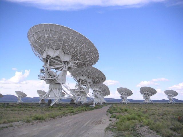
1 Introduction, Unix, C++
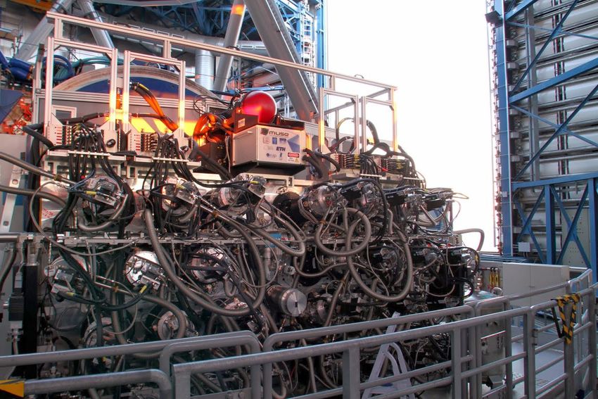
Integral Field Spectrographs like the Multi-Unit Spectroscopic Explorer (MUSE) at the
Very Large Telescope (VLT) in Chile split the field of view into small slices (up to 24 × 48
for MUSE) and disperse them in a spectrograph and record these spectra with a CCD
(24 individual spectrographs and CCDs for MUSE). A computer has to synchronize all
these components and process the raw data to obtain a multi-wavelength image. MUSE
also highly profits by the Adaptive Optics (AO) of the Yepun telescope (UT4). This
AO tries to get rid of image blurring from atmospheric turbulences by deforming the
secondary mirror very fast to reduce the effect of incoming light wavefront distortions.
Doing so, the spatial resolution can be as good as when observing with the Hubble Space
Telescope (HST). As the HST is out of reach in the orbit (≈ 500 km height), it must
perform many operations autonomously with help of the onboard computer like the Intel
486.
The radio regime has become more and more important in the last decades, modern
radio telescopes consist of many small antennae, covering large parts of Earth’s surface.
However, radio telescopes cannot directly map the sources. Instead computers have to
combine the signals of these many antennae to compute an image with spatial informa-
tion.
Figure 1.1: MUSE, VLA, HST
Computers are also necessary for data analysis or data reduction (the process of getting,
e.g., a calibrated optical spectrum from a CCD raw image), starting with processing the
individual exposures from, e.g., MUSE, to combine them finally to a 3dCube, containing
spectral and spatial information. Such data are usually stored in the Flexible Image
Transport System (FITS) format. If data are recorded in a times series, a search for
periodicity hidden in the data by Fourier analysis can reveal pulsations or rotation of an
object.
10 1%
10%
P N (ω)
50%
5
0
0.0 0.5 1.0 1.5 2.0 2.5 3.0
ω [s -1 ]
Figure 1.2: IDL, 3dCube / FITS, Fourier analysis
6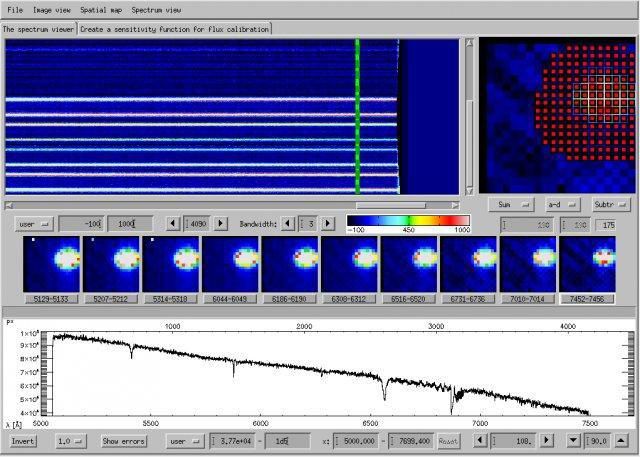
1.2 About computers
The showcase in the field for the use of computers are of course the numerical simu-
lations or modelling. The largest simulations comprise the whole universe in a box of
3.7 Gpc edge length, running on a super computer with 12 000 CPU cores and 30 TiB
memory. This Millenium XXL simulation belongs to the class of N -body simulations,
suiteable if gravity is the main driver. Going to smaller scales requires the inclusion
of hydrodynamics. Many different approaches exist for this field of computational as-
trophysics and are the topic of the lecture “Computationl Astrophysics II” in the next
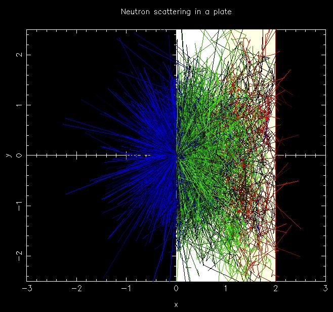
semester. If scattering processes play an important role, it is often easier and more flexi-
ble to use Monte-Carlo (MC) techniques. We will study the neutron transport with help
of MC simulations.
Figure 1.3: N-body simulation, hydrodynamics , Monte-Carlo
1.2 About computers
Many stories about the history of computers begin with the abacus, a calculation tool
already used more than 3000 years ago in Mesopoatamian. However, this tool has more
in common with paper and pen than with a real computer.
So, the real history of computer started with the combination of a computer unit and
memory – something that all the precursors of the computer lacked – to have a fully
programmable device. The ability to be programmed is often understood in a strict way,
that the programming language used on the computer is Turing complete 1
The first devices that can be called a computer were the electromechanical Z3 by Kon-
rad Zuse2 in Berlin, 1941; the electronic Colossus computer by Thomas Harold Flowers3
in London, 1943 – although it was not Turing complete; and the Electronic Numerical
Integrator and Computer (ENIAC ) by the University of Pennsylvania from 1945. ENIAC
was already 1000 times faster than electromechanical computers, but it could not perfom
floating point operations.
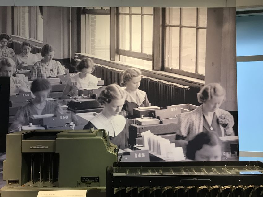
The development of computers was accompanied by the success of punched cards in
the 1950’s, used for the storage and structure of large datasets, e.g., for the “Atlas of the
British Flora” (see Fig. 1.4). The extensive use of punched cards started already much
earlier with the United States Census of 1890, using the punched cards methods invented
1
Alan Turing, 23.06.1912-07.06.1954, England
2
Konrad Zuse, 22.06.1910-18.12.1995, Germany
3
Thomas Harold Flowers, 22.12.1905-28.10.1998, England
7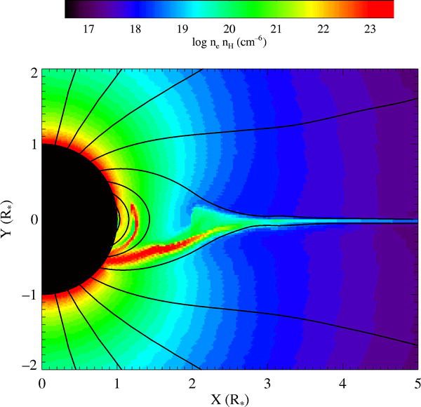
1 Introduction, Unix, C++

Figure 1.4: IBM 77 electric punched cards collator (1937-1957) in the Computer History
Museum in Mountain View, USA. In the background IT stuff handles punched cards.
Until the advent of modern software in the 1960s, programming was mainly done by
women.

by Herman Hollerith4 . Punched cards were the main computer input and storage medium
until the 1970s. We will later see how this has influenced the first high-level programming
languages.
   While in principal computers could use any numeral (positional) system, especially the
common decimal system as used by ENIAC, the binary numeral system was established
for practical reasons, and already used by the Z3 : There are only two states (0 and 1) that
a device must distinguish. This is much easier and robust to implement in electronics: 0
is below some threshold voltage, and 1 is above it.
   Most modern standards for computing are based on the work of the Institute of Elec-
trical and Electronics Engineers (IEEE), founded in 1963 in the USA. These standards
comprise, e.g., the floating-point arithmetic (IEEE 754), the Ethernet (IEEE 802.3), or
the Portable Operating System Interface (POSIX, IEEE 1003) for Unix and other oper-
ating systems.

 4
     Herman Hollerith, 29.02.1860-17.11.1929, USA

8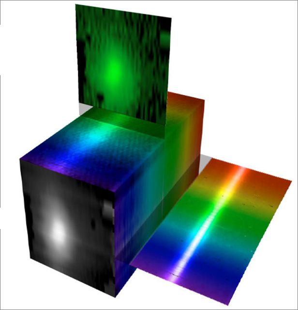
1.2 About computers

1.2.1 Components of a computer

The “atoms” from which a computer is built are the logic gates. A logic gate is a hardware
realization, i.e. made of silicon transistors and diodes (or vacuum tubes for the first
computers), of a boolean5 or logical function. For example the AND gate:

Table 1.2: Truth table for the boolean func-                       A
tion AND
                   input    output                                 B
                   A B        Q                                                Q

                   0    0       0
                   0    1       0
                   1    0       0                                  A
                                                                                   Q
                   1    1       1                                  B

                                                    Figure 1.5: AND gate realized with two npn
                                                    transistors and its IEEE symbol

  Most modern gates are made from metal-oxide-semiconductor field-effect transistors
(MOSFET), as they are cheap and can be highly packed. Logic gates can be combined
to perform more elaborated operations: E.g. the parallel connection of an AND gate and
an XOR (exclusive or) gate acts as a half adder for two single binary digits A and B.
The output of the XOR gate gives the sum (S), while the AND gate delivers the carry
(C):

Table 1.3: Half adder, truth table for AND                     A
                                                                         XOR           S
(C) and for exclusive or XOR (S)                               B

                   input    output
                   A B      C S                                          AND           C

                   0    0   0       0
                   0    1   0       1
                   1    0   0       1               Figure 1.6: A halfer adder realized through
                   1    1   1       1               parallel AND and XOR gate

Further combinations of logic gates yield, e.g., arithmetic logic units (ALU) in the pro-
cessors; flip-flop circuits for the registers (see Fig. 1.7), that are fast, but small memory
units in the processors; and together with capacitors the computer memory for data
storage (Random Access Memory, RAM).

 5
     George Boole, 02.11.1815-08.12.1864, England

                                                                                             9
1 Introduction, Unix, C++
S
NOR 2 Q
Table 1.4: Truth table for a simple flip-flop,
R=S=1 is not allowed, while R=S=0 allows
read-out (hold state)
state S R output NOR 1 Q
R
(previous Q) (state) (reset) next Q
0 0 0 0
0 0 1 0 Figure 1.7: A simple storage, called flipflop,
0 1 0 1 realized with two NOR gates. Note the
1 0 0 1 feedback circuit, which has to stable modes.
1 1 0 1 This device can be further improved by
1 0 1 0 adding a second level of gates with a clock
signal.
The Central Processing Unit
The Central Processing Unit (CPU) of a modern computer consists of hundreds of mil-
lions of logic gates, summing up to, e.g., 38.4 billion transistors for a 64 core AMD Ryzen
Threadripper 3990X (high end) desktop CPU. The typical size of a transistor in the CPU
is 7 nm and such CPUs can be found in normal (high end) desktop computers. For com-
parison: ENIAC from 75 years ago contained 20 000 vacuum tubes, each had a size of
several cm. It was first estimated by Gordon Moore6 that the number of transistors in
a CPU doubles every two years (Moore’s law) due to improvement in the production
process.
The performance of a CPU can be expressed in floating point operations per second
(FLOPS) and is determined by the size of its registers and caches, its architecture (e.g.,
out-of-order execution, pipelining), its number of cores, and its clock rate. The latter
one is given in GHz. Within the same processor family, a higher clock rate usually scales
with the performance of the CPU, meaning that a 4.1 GHz CPU is about 8% faster than
a 3.8 GHz CPU of the same type. A clock cycle is the time the electronic circuits of the
CPU need to settle their new state (0 or 1). The higher the quality of the integrated
circuits, the faster this transition can happen and the higher can be the CPU frequency.
Note that many operations need more than one clock cycle, e.g., dividing to float
numbers needs more than twice the number of cycles than multiplication. As modern
CPUs can vary their clock rate over a large range depending on the thermal budget
(heat losses), the usually given base CPU frequency cannot longer be used to compare
the performance of CPUs. Instead, one has to run benchmark programms, like the
LINPACK benchmark, which is used to compare supercomputers:
6
Gordon Moore, 03.01.1929, USA
101.2 About computers
Computer/CPU FLOPS cores year ref.
Z3 2 (adding) 1 1941
AMD Ryzen 3990X 1.6 × 1012 64 2020 Link
Summit (USA) 149 × 1015 202 752 + GPUs 2020
Memory
Due to technical and economic constraints, a computer has basically two different kinds
of memory or storage:
1. fast, but expensive and volatile memory for the actual processing, e.g., CPU caches,
RAM (5 Euro/GB)
2. very slow, but permanent and cheap memory for storage, e.g., HDD (Hard Disk
Drive, 3 Cent/GB), SDD (Solid State Drive, 15 Cent/GB)
Usually, the amount of the volatile memory is much smaller than those of the permanent
memory, therefore the permanent memory is also referred to as mass storage. RAM
comes in GB, HDD in TB. The early computers used punched cards or magnetic tapes
for mass storage, modern computers use magnetic disks in RAIDs (Redundant Array of
Independent/Inexpensive Disks), optical discs (CD-ROM, DVD, . . . ), or silicon based
devices like SSDs.
When accessing memory the computer has first to locate the data, e.g., compute an
absolute address, and then to read it in. In some designs, like General-purpose computing
on graphics processing units (GPGPU), where the fast processors have a high throughput,
the data access becomes indeed the bottleneck and causes latencies (see Tab. 1.5). When
transitioning to multithreading programming, that is also something one has to have in
mind, the time penalties for copying data to the individual threads.
Table 1.5: Latencies of memory operations in relation to each other, see github
operation real time scaled time (×109 )
Level 1 cache access 0.5 ns 0.5 s (∼ heart beat)
Level 2 cache access 7 ns 7s
Multiply two floats 10 ns 10 s (estimated)
RAM access 100 ns 1.5 min
Send 2kB over Gigabit network 20 000 ns 5.5 h
Read 1MB from RAM 250 000 ns 2.9 d
Read 1MB from SSD 1 000 000 ns 11.6 d
Read 1MB from HDD 20 000 000 ns 7.8 months
Send packet DE→ US→ DE 150 000 000 ns 4.8 years
111 Introduction, Unix, C++
One should know these numbers when starting with High Performance Computing. If
data and program code fit in the cache, they can be executed much much faster. Also,
these numbers refer to sequential read, if the computer first has to seek fragmented data
on the disk, it will take even longer.
Unfortunately, many ways of modern elegant programming (recursion, templates,
classes) are contrary to the way computer hardware works, i.e. they just slow down pro-
gram execution. Therefore, we will focus on a more “traditional” way of programming,
so, we prefer a C-style C++ and will later learn why Fortran can be faster. In fact,
the LINPACK benchmark for the TOP 500 list of supercomputers is originally written
in Fortran.
1.3 The stud domain and cluster
1.3.1 The computer lab
Unix/Linux is a multi-user operating system, therefore every user needs his own user
account. The stud domain (stud.physik.uni-potsdam.de) is a little cluster of 17 NFS
(Network File System) mounted Linux computers running on openSuSE 15.1. There are
several Intel Core i7-2600K, i7-4770, i7-7700, i7-8700 desktops, and 1 Xeon Gold 6152
44 -core compute server. These computers can be accessed in the computer lab rooms
0.087 (for lectures only) and 1.100 (for students). The computers in room 0.087 have a
(local) guest accout, which cannot be accessed from outside. Therefore, please get your
own account (user name and password).
Attention: Unix/Linux is case sensitive!
Hint: You can choose the session type (e.g., Xfce, IceWM) at the login screen.
Security advice
As soon as you got your own account:
passwd Change the user password
(Enter the command in a terminal, Xterm, Konsole, or similar.)
Change your initial NIS password(!) to a strong password, use
• at least 9 characters, comprising of:
• capital AND lowercase letters, but not single words
• AND numbers
• AND special characters (Attention! Mind the keyboard layout!)
e.g., $cPhT-25@comP2 or tea4Pollen+Ahead
The initial password expires after 14 days.
121.3 The stud domain and cluster
The computers in the computer lab rooms are always on, as they are accessed from
outside via ssh, perform long-term calculations, and serve as file servers for the user
directories. The hosts bell, mahler, and weber contain your home directories physically
on their disks and act as NFS servers. Therefore, it doesn’t matter on which computer of
the cluster you login with your accout, you can always access your own home directory.
Each home directory has a quota of 200 GB.
1.3.2 Linux
Linux is a derivative of the operating system Unix. It is a multi-user and multitasking
operating system. It was written in 1991 by Linux Torvalds as a Unix for PCs, now it is
available for (almost) every platform, e.g., as Android or in Wireless routers. It is under
permanent development. Linux is
• for free
• open source (program code can also be modified)
• the combination of a monolithic kernel (maintained by Linus Torvalds and devel-
opers) and (GNU) software
• dominant in supercomputers (more than 90%).
Nowadays there are numerous Linux distributions, mostly differing by their installation
and administration tools, e.g., Ubuntu, Fedora, openSuSE.
Graphical desktop environments
Important X-Window based environments under Linux are GNOME, KDE, Xfce, ICEWM.
Xfce and ICEWM are light-weighted environements and therefore available on the com-
puters of the cluster. The desktop environment (session type) can be chosen during
local(!) login. Do not confuse desktop environment and Linux distribution. Although
some Linux distribution prefer a specific window manager (Kubuntu with KDE), it is
usually possible to install other window mangers and use them.
Important tools/programs
The most basic and also most powerfull tool in Unix/Linux is the terminal, which comes
in different flavors. The xterm is very simple(!) and fast. There are more comfortable
kinds of terminals, like konsole, allowing for multiple tabs or different color/font schemes.
The terminal is only the vehicle for another program, which runs in a terminal and is
called the shell. The shell is used to enter Linux commands, like cd or ls. There are
also different types of shell. The most important one are the csh (C Shell) and the
bash (Bourne-Again Shell). We will use the terminal/shell for compiling and running
our programs.
131 Introduction, Unix, C++
Task 1.3.1 Terminal
Open a terminal, Xterm, konsole, or similar.
We will also use an editor for pure (ASCII) text files to write the source code, e.g.,
hello.cp. Although the number of editors is large and constantly increasing, it is rec-
ommended to choose – after some testing of different editors – one editor and stay with
it for the rest of your life.
Usually one has to make a trade-off between convenience, speed, and availability:
vi/vim : Available on every Unix/Linux system, text-based (does not need graphical
window). The vi uses two different modes:
i insert input mode (text input)
a append input mode (text input)
change to command mode:
:w write file, in command mode
:q! quit without further questions, in command mode
x delete one character, in command mode
dd delete whole line, in command mode
Task 1.3.2 vi
1. Start vi and give at the same time as argument the name of a file, e.g., your
first name. For example: vi helge.txt
2. Change to the input mode and enter the following text: “Hellow, world!”
3. Save the file and quit the vi.
emacs : can be installed on every Unix/Linux sytem, MacOS X, Windows, text-based
(emacs -nw ) and window-based mode supported. The commands are entered with help
of the key and the key. In the following tables a plus + means that both
keys must be pressed at the same time, otherwise subsequently.
+ x + c close (quit)
+ x + s save (write)
+ k kill (cut from cursor position till end of line)
+ y yank (paste)
+ mark
+ w cut marked area
14 w copy marked area1.4 Shell and shell
Task 1.3.3 emacs
1. Use emacs to open the text file, previously crated with vi. Start emacs in
the background by appending the ampersand &, i.e., emacs helge.txt &
2. Copy the first text line with help of the kill command and clone this line.
3. Save the result and quit emacs.
kate : can be installed on every Linux system that supports KDE, windowbased.
+ c copy marked area
+ v paste copied area
+ s save
+ q quit
In the submenu Edit → Block Selection Mode allows to mark columns (instead of
lines).
Task 1.3.4 kate
1. If not already done so, open an Xterm.
2. Type in cal to display the calendar for the current month. Copy this calendar
output into the mouse buffer. In Linux: just mark the calendar by pressing
the left mouse button, it is automatically inserted to the mouse buffer. Mac
OS X: You have to press additionally CMD + c.
3. Start kate in the background (&) and insert the calendar text from the
mouse button: Linux: just press the middle mouse button. Mac OS X: Press
CMD + v.
4. Delete the column with the Mondays by marking the corresponding column.
5. Save the result and quit kate.
Compilers We will use the command-line compilers g++, gfortran, and ifort. Their
usage is explained in the next chapter.
1.4 Shell and shell
Unix provides by the shell (command line) an extremely powerful tool. Within the shell
Unix commands are executed.
151 Introduction, Unix, C++
Unix command syntax
command [-option] [argument]
Attention! Mind the blanks!
As blanks (one ore multiple) are used in the shell to separate the list of options and
arguments, which can be file names, it is strictly recommended to avoid blanks in file
names! Although blanks in file names are possible, it just makes everything more com-
plicated.
Task 1.4.1 Shell commands
Open an xterm or similar terminal/console and enter following: (finish each line
with ):
echo hello
and
echo -n hello
What’s the difference?
Command history
By ↑ (arrow key up) you can repeat the last commands entered in the shell.
A list of the last commands can be shown via the command
history
Moreover, you can save typing by using the TAB key, it completes commands or file
names:
ec
is completed to
echo
1.4.1 Directories
The filesystem tree In Linux, there is only one root directory / per computer. All
devices (disks, drives, etc.) are shown below this / as devices in /dev/ or accessible as
directories through the process of mounting.
161.4 Shell and shell
/
| → root of the FS tree
|-- /home/
| | → Home directories
| |-- /home/weber/
| | → Homes on weber
| |--/home/weber/htodt/
→ Helge’s home
|
|
|-- /etc/ → et cetera (config)
|
|
|-- /dev/ → devices
Navigation through directories Although one can use a file manager, it is much faster
to navigate through the file tree by using simple shell commands:
pwd shows the current directory path (absolute)
e.g., /home/weber/htodt
cd name change to directory name
. means the current directory
.. the parent directory, e.g., cd ..
/ root of the FS tree
∼ the home directory, e.g., cd ∼ or just cd
∼user the home directory of user
Moreover, one can easily create or delete directories with the corresponding shell com-
mands. One of the most often used commands is ls, which displays the content of the
given directory (argument). If no argument is given, it shows the content of the current
directory.
mkdir name create directory name
rmdir name remove directory name
ls show (list) the content of the directory
The command ls has some options, which you should also know:
171 Introduction, Unix, C++
ls show the content of the current directory
ls -a also show hidden files (starting with a .)
ls -l show the file attributes, owner, creation time
In a Unix/Linux file system, all files are saved together with some additional informa-
tion, the so-called file attributes, which contain the ownership, time stamps, and access
permissons of the file. Some file systems also store extended attributes.
File attributes
drwxr-xr-x 2 htodt users 4096 14. Oct 13:35 Documents
d = directory r = readable
w = writeable x = executable
htodt = owner users = group
4096 = size in byte 14. Oct 13:35 = creation time
Documents = name of the file (here: of the directory)
Hint: ls -lc shows the time of last modification ; ls -lu shows the time of last access
(e.g., read), if supported by file system.
There exist several possibilities to obtain help/information for a specific shell command,
i.e., which options are supported:
man ls Manual pages (help for the command ls)
info ls Info pages (alternative help for the command ls)
ls −−help Help for the command ls
ls −−help | less if more than one screen page
Navigation through man pages – also less and more
q quit
next page b previous page
/ forward search ? backward search
n next occurrence N previous occurrence
> jump to the end < jump to the beginning
18You can also read