Learning to Play Games IEEE CIG 2008 Tutorial - Simon M. Lucas University of Essex, UK
←
→
Page content transcription
If your browser does not render page correctly, please read the page content below
Learning to Play Games
 IEEE CIG 2008 Tutorial

    Simon M. Lucas
 University of Essex, UK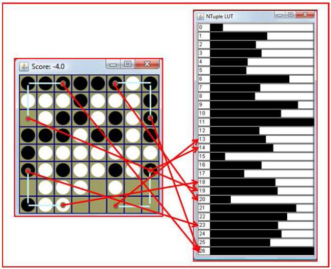
Aims
• To provide a practical guide to the main machine
  learning methods used to learn game strategy
• Provide insights into when each method is likely to
  work best
   – Details can mean difference between success and failure
• Common problems, and some solutions
• We assume you are familiar with
   – Neural networks: MLPs and Back‐Propagation
   – Rudiments of evolutionary algorithms (evaluation,
     selection, reproduction/variation)
• Demonstrate TDL and Evolution in action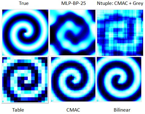
Overview
• Architecture (action selector v. value function)
• Learning algorithm (Evolution v. Temporal
  Difference Learning)
• Function approximation method
  – E.g. MLP or Table Function
  – Interpolated tables
• Information rates
• Sample games (Mountain Car, Othello, Ms. Pac‐
  Man)
Architecture
• Where does the computational intelligence fit
  in to a game playing agent?
• Two main choices
  – Value function
  – Action selector
• First, let’s see how this works in a simple grid
  world
Action Selector
• Maps observed current game state to desired
  action
• For
  – No need for internal game model
  – Fast operation when trained
• Against
  – More training iterations needed (more parameters to
    set)
  – May need filtering to produce legal actions
  – Separate actuators may need to be coordinated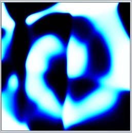
State Value Function
• Hypothetically apply possible actions to current
  state to generate set of possible next states
• Evaluate these using value function
• Pick the action that leads to the most favourable
  state
• For
  – Easy to apply, learns relatively quickly
• Against
  – Need a model of the system
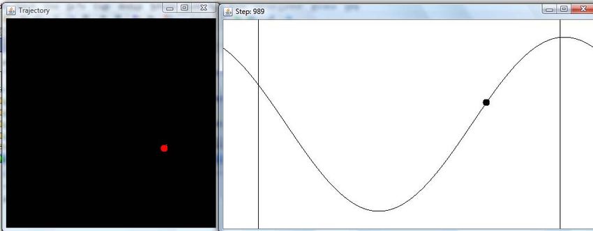
Grid World
• n x n grid (toroidal i.e. wrap‐around)
• Reward: 0 at goal, ‐1 elsewhere
• State: current square {i, j}
• Actions: up, down, left, right
• Red Disc: current state
• Red circles: possible next states
• Each episode: start at random place
  on grid and take actions according to
  policy until the goal is reached, or
  maximum iterations have been
  reached
• Examples below use 15 x 15 grid
State Value versus
  State‐Action Value: Grid World Example
• State value: consider the four
  states reachable from the
  current state by the set of
  possible actions
   – choose action that leads to highest
     value state
• State‐Action Value
   – Take the action that has the
     highest value given the current
     state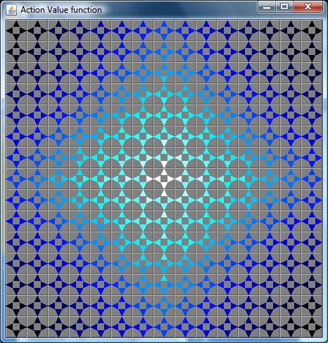
Run Demo:
Time to see each approach in action

Learning Algorithm:
                (Co) Evolution v. TDL
• Temporal Difference Learning
   –   Often learns much faster
   –   But less robust
   –   Learns during game‐play
   –   Uses information readily available (i.e. current
       observable game‐state)
• Evolution / Co‐evolution (vanilla form)
   – Information from game result(s)
   – Easier to apply
   – But wasteful: discards so much information
• Both can learn game strategy from scratch
Co‐evolution (single population) Evolutionary algorithm: rank them using a league
In Pictures…
Information Flow
• Interesting to observe information flow
• Simulating games can be expensive
• Want to make the most of that computational
  effort
• Interesting to consider bounds on information
  gained per episode (e.g. per game)
• Consider upper bounds
  – All events considered equiprobable
Evolution
• Suppose we run a co‐evolution league with 30
  players in a round robin league (each playing
  home and away)
• Need n(n‐1) games
• Single parent: pick one from n
• log_2(n)
• Information rate:
TDL
• Information is fed back as follows:
   – 1.6 bits at end of game (win/lose/draw)
• In Othello, 60 moves
• Average branching factor of 7
   – 2.8 bits of information per move
   – 60 * 2.8 = 168
• Therefore:
   – Up to nearly 170 bits per game (> 20,000 times more than
     coevolution for this scenario)
   – (this bound is very loose – why?)
• See my CIG 2008 paper
Sample TDL Algorithm: TD(0)
typical alpha: 0.1
pi: policy; choose rand move 10% of time
else choose best stateMain Software Modules
(my setup – plug in game of choice)
Game
Problem Game
Agent
Adapter Engine
Controller
Vector Value
Vectoriser TDL
Optimiser Function
ES EDA Radial
Interpolated
MLP Basis
Table
FunctionFunction Approximators • For small games (e.g. OXO) game state is so small that state values can be stored directly in a table • Our focus is on more complex games, where this is simply not possible e.g. – Discrete but large (Chess, Go, Othello, Pac‐Man) – Continuous (Mountain Car, Halo, Car racing: TORCS) • Therefore necessary to use a function approximation technique
Function Approximators
• Multi‐Layer Perceptrons (MLPs)
– Very general
– Can cope with high‐dimensional input
– Global nature can make forgetting a problem
• N‐Tuple systems
– Good for discrete inputs (e.g. board games)
– Harder to apply to continuous domains
• Table‐based
– Naïve is poor for continuous domains
– CMAC coding improves this (overlapping tiles)
– Even better: use interpolated tables
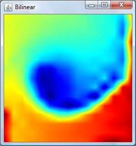
• Generalisation of bilinear interpolation used in image transformsStandard (left) versus CMAC (right)
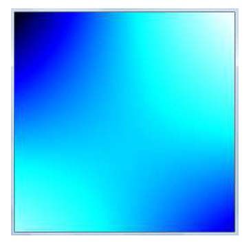
Interpolated Table
Method
• Continuous point p(x,y)
• x and y are discretised, then residues r(x) r(y)
  are used to interpolate between values at four
  corner points
• N‐dimensional table requires 2^n lookups
Supervised Training Test
• Following based on 50,000 one‐shot training
  samples
• Each point randomly chosen from uniform
  distribution over input space
• Function to learn: continuous spiral (r and
  theta are the polar coordinates of x and y)
Results

          MLP‐CMAES
Test Set MSE
Standard Regression
              200 Training Points
           Gaussian Processes Model
     Data set           Interpolated Table   Gaussian Processes

Gaussian Processes: learn more from the data, but hard to
interface to games
Function Approximator: Adaptation Demo This shows each method after a single presentation of each of six patterns, three positive, three negative. What do you notice?
Grid World – Evolved MLP
• MLP evolved using
  CMA‐ES
• Gets close to optimal
  after a few thousand
  fitness evaluations
• Each one based on 10
  or 20 episodes
• Value functions may
  differ from run to run
Evolved N‐Linear Table
• This was evolved
  using CMA‐ES, but
  only had a fitness of
  around 80
Evolved N‐Linear Table
      with Lamarkian TD‐Learning
• This does better
• Average score now
  8.4
                  Evo N‐Linear 5
TDL Again • Note how quickly it converges with the small grid
TDL MLP
• Surprisingly hard to
  make it work!
Table Function TDL
                 (15 x 15)
• Typical score of 11.0
• Not as good as
  interpolated 5 x 5
  table on this task
• Model selection is
  important
Grid World Results – State Table • Interesting! • The MLP / TDL combination is very poor • Evolution with MLP gets close to TDL with N‐Linear table, but at much greater computational cost Architecture Evolution (CMA‐ES) TDL(0) MLP (15 hidden units) 9.0 126.0 N‐Linear Table (5 x 5) 11.0 8.4
Action Values ‐ Takes longer
e.g. score of 9.8 after 4,000 episodes
Simple Example: Mountain Car
• Standard reinforcement learning benchmark
• Accelerate a car to reach goal at top of incline
• Engine force weaker than gravity
Value Functions Learned (TDL)
Mountain Car Results
(TDL, 2000 episodes, ave. of 10 runs)
       System        Mean steps to goal (s.e.)

        Table               1008 (143)

    CMAC: separate          81.8 (11.5)

     CMAC: shared           60.0 (2.3)

       Bilinear             50.5 (2.5)
Othello See Demo
Volatile Piece Difference

          move
            Move
Setup • Use weighted piece counter – Fast to compute (can play billions of games) – Easy to visualise – See if we can beat the ‘standard’ weights • Limit search depth to 1‐ply – Enables billions of games to be played – For a thorough comparison • Focus on machine learning rather than game‐tree search • Force random moves (with prob. 0.1) – Get a more robust evaluation of playing ability
Othello: After‐state Value Function
Standard “Heuristic” Weights
(lighter = more advantageous)
TDL Algorithm
• Nearly as simple to apply as CEL
public interface TDLPlayer extends Player {
    void inGameUpdate(double[] prev, double[] next);

    void terminalUpdate(double[] prev, double tg);

}

• Reward signal only given at game end
• Initial alpha and alpha cooling rate tuned
  empirically
TDL in Java
CEL Algorithm
• Evolution Strategy (ES)
  – (1, 10) (non‐elitist worked best)
• Gaussian mutation
  – Fixed sigma (not adaptive)
  – Fixed works just as well here
• Fitness defined by full round‐robin league
  performance (e.g. 1, 0, ‐1 for w/d/l)
• Parent child averaging
  – Defeats noise inherent in fitness evaluation
Algorithm in detail
(Lucas and Runarsson, CIG 2006)
CEL (1,10) v. Heuristic
TDL v. Random and Heuristic
Othello: Symmetry
• Enforce symmetry
  – This speeds up learning

• Use trusty old friend: N‐Tuple System for value
  approximator
NTuple Systems
• W. Bledsoe and I. Browning. Pattern recognition and
reading by machine. In Proceedings of the EJCC, pages 225
232, December 1959.
• Sample n‐tuples of input space
• Map sampled values to memory indexes
– Training: adjust values there
– Recognition / play: sum over the values
• Superfast
• Related to:
– Kernel trick of SVM (non‐linear map to high dimensional space;
then linear model)
– Kanerva’s sparse memory model
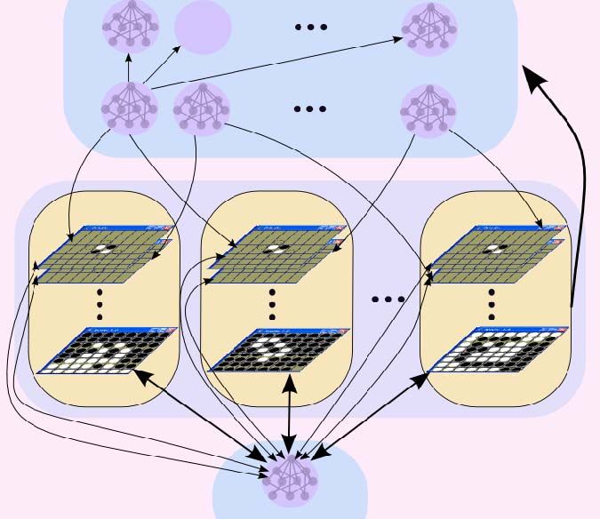
– Also similar to Michael Buro’s look‐up table for LogistelloSymmetric 3‐tuple Example
Symmetric N‐Tuple Sampling
N‐Tuple System
• Results used 30 random n‐tuples
• Snakes created by a random 6‐step walk
  – Duplicates squares deleted
• System typically has around 15000 weights
• Simple training rule:
N‐Tuple Training Algorithm
NTuple System (TDL)
      total games = 1250
(very competitive performance)
Typical Learned strategy…
(N‐Tuple player is +ve – 10 sample games
shown)Web‐based League
(May 15th 2008)
All Leading entries are N‐Tuple basedResults versus CEC 2006 Champion (a manual EVO / TDL hybrid MLP)
N‐Tuple Summary
• Stunning results compared to other game‐
  learning architectures such as MLP
• How might this hold for other problems?
• How easy are N‐Tuples to apply to other
  domains?
Ms Pac‐Man
• Challenging Game
• Discrete but large
  search space
• Need to code inputs
  before applying to
  function
  approximator
Screen Capture Mode
• Allows us to
  run software
  agents original
  game
• But simulated
  copy (previous
  slide) is much
  faster, and
  good for
  training
Ms Pac‐Man Input Coding
• See groups of 4 features below
• These are displayed for each possible
  successor node from the current node
  – Distance to nearest ghost
  – Distance to nearest edible ghost
  – Distance to nearest food pill
  – Distance to nearest power pill
Alternative Pac‐Man Features
             (Pete Burrow)
• Used a smaller feature space
• Distance to nearest safe junction
• Distance to nearest pill
So far: Evolved MLP by far the best!
Results: MLP versus Interpolated Table
• Both used a 1+9 ES, run for 50 generations
• 10 games per fitness evaluation
• 10 complete runs of each architecture
• MLP had 5 hidden units
• Interpolated table had 3^4 entries
• So far each had a mean best score of approx
  3,700
• More work is needed to improve this
    – And to test transference to original game!
Summary
• All choices need careful investigation
– Big impact on performance
• Function approximator
– N‐Tuples and interpolated tables: very promising
– Table‐based methods often learn much more reliably than MLPs
(especially with TDL)
– But: Evolved MLP better on Ms Pac‐Man
• Input features need more design effort…
• Learning algorithm
– TDL is often better for large numbers of parameters
– But TDL may perform poorly with MLPs
– Evolution is easier to apply
• Some things work very well, though much more research
needed
• This is good news!New Transactions
You can also read