Comparison of Luminous Intensity Distributions

15. Internationales Forum für den lichttechnischen Nachwuchs
 Ilmenau, 04. – 06. Juni 2021
 DOI (proceedings): 10.22032/dbt.48427
DOI: 10.22032/dbt.49322

 Comparison of Luminous Intensity Distributions

Lerch, David; Trampert, Klaus; Neumann, Cornelius
Karlsruher Institute for Technology (KIT), Light Technology Institute (LTI)
Engesserstraße 13, Geb. 30.34, 76131 Karlsruhe
Tel. 0721 608-47383, david.lerch@kit.edu, www.lti.kit.edu

Abstract
If headlights for automobiles are put on the market, legal requirements must be
complied with. Whether the oncoming traffic is dazzled by the headlights can be
determined from the luminous intensity distribution curve (LID). For this, the so-called
cut-off line must be determined. A declaration of conformity is only possible if the
uncertainties of all sizes are considered.
A measured value in the LID consists of a direction, the solid angle, and an amount,
the luminous intensity. If you represent each value of the LID as a vector and
interpolate the support points, you get the luminous intensity body. When comparing
LIDs according to the prior art, the luminous intensities are compared in pairs for each
solid angle.
During a measurement, the position of the object in the measurement coordinate
system is unknown, for example due to misalignment. As a result, the object coordinate
system is shifted to the measurement coordinate system and a pairwise comparison is
not expedient for each spatial direction.
If LIDs are compared on the basis of the intrinsic properties of the LID body, the
orientation of the LID can be found in the measurement coordinate system. The aim of
this work is to compare two LIDs based on the intrinsic properties of the LID body.

© 2021 by the authors. – Licensee Technische Universität llmenau, Deutschland.
 This is an Open Access article distributed under the terms of the
 Creative Commons Attribution ShareAlike-4.0 International License,
 (https://creativecommons.org/licenses/by-sa/4.0/). - 121 -

15. Forum für den lichttechnischen Nachwuchs
 Ilmenau, 04 – 06 Juni 2021

1 Motivation
In this work an approach is developed with which light distribution curves (LID) of the
same luminaire are compared with one another. If two identical luminaires from
different laboratories are to be measured, it is difficult to compare the two
measurements.
When measuring a LID in the far field, it is important to know the exact center of light
of the luminaire to be measured. It could be shown that the position of the center of
light during a measurement has a great influence on the photometric limit distance [5].
In addition, it was found that the greatest uncertainty contribution to the orientation
between light source and receiver during a measurement is the uncertainty of the
orientation of the light source [4].
For the development of a method with which LIDs can be compared whose luminaires
are the same but are oriented differently during the measurement, measurements are
required in which a luminaire is measured in different orientations.
Measuring different luminaires for different orientations is very time consuming. A LID
generator is therefore to be developed with which luminaires can be measured
virtually.

2 Related work

2.1 Synthetic LIDs
There have been publications on LID generators in the past. The LITG has published
software, developed by Dipl.-Ing. Nils Haferkemper, with which the resulting light
distribution can be obtained for a certain room geometry, position and geometry of the
luminaire and illuminance [3]. This LID generator was developed for developers and
users of light simulation programs. As part of this work, a generator is developed that
has been optimized for metrological applications.

2.2 Comparison of LIDs
In recent years, the point-to-point comparison of measured values has become
established for the comparison of LIDs. When comparing the LIDs of two identical
luminaires, it is known that the LIDs to be compared are ideally identical.
This basic assumption enables an optimization approach in which the distance
between the two LIDs is minimized. For this, one LID is chosen as a reference, while
the second is the test LID.
Now the test LID is shifted so that the distance between the two LIDs is minimal. Due
to the shift, the test LID requires values that lie between the measured values. These
intermediate values are obtained by means of linear interpolation between the
measured values [1, 2].

© 2021 by the authors. – Licensee Technische Universität llmenau, Deutschland. - 122 -

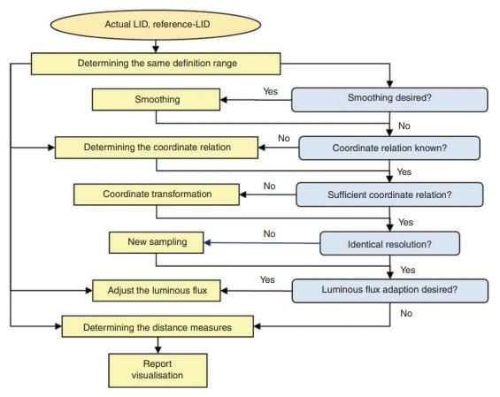
15. Forum für den lichttechnischen Nachwuchs
 Ilmenau, 04 – 06 Juni 2021

The optimization can be done by means of a systematic shift [1] with constant steps,
or with the minimization of the quadratic error [2]. In Figure 1 a flow chart is presented
that shows which preprocessing steps are necessary in order to compare the light
distributions with one another.

 Figure 1: Flow chart for the comparison of LIDs [2]

© 2021 by the authors. – Licensee Technische Universität llmenau, Deutschland. - 123 -

15. Forum für den lichttechnischen Nachwuchs
 Ilmenau, 04 – 06 Juni 2021

3 Implementation
As part of this work, a framework was developed with which synthetic light distributions
can be generated and measured virtually. For the artificial light distributions, analytical
models were set up with which real light distributions can be approximated.
Furthermore, features of LIDs are introduced.

3.1 Synthetic LIDs
In this work, a synthetic light distribution is composed of so-called cosine lobes. The
shape of a cosine lobe is ( ( )), with the form factor of the radiation
characteristic and the tilting angle of the lobe. For each lobe a luminous flux 
is determined. For each radiation direction the luminous intensity is:
 ( )
 = ∑ ∗ (3.1)
 ′
 
With:
 ′ sin ′ cos ′
 ( ′ ) = ( sin ′ sin ′ ) (3.2)
 ′ cos ′
 ′
 ( ) = ( ′ ) (3.3)
 ′
 = ( ) ( ) ( ) =
 cos cos − sin cos sin − cos sin − sin cos cos sin sin 
 (sin cos + cos cos sin − sin sin + cos cos cos − cos sin ) (3.4)
 sin sin sin cos cos 
 = , = , = 
 
 = (3.6)
 √ 2 + √ 2 + √ 2

 ′ = ∑ ( ) ∗ (3.7)
 
A synthetic light distribution can then be measured virtually. The C-plane system is
used as the measuring coordinate system. To simplify the rotation, the coordinates of
the C-plane system are converted into Cartesian coordinates and the rotations are
carried out there.
This is followed by a reverse transformation into the C-level system. The optical axis
points in the positive z-direction. The resolution of the measurement can be chosen
arbitrarily.

© 2021 by the authors. – Licensee Technische Universität llmenau, Deutschland. - 124 -

15. Forum für den lichttechnischen Nachwuchs
 Ilmenau, 04 – 06 Juni 2021

In order to simulate squinting of the lamp, the measurement coordinate system is
rotated on a spherical surface. For this, the formula (3.3) is extended by the rotation
matrix Rm:
 ′
 ( ) = ( ′ ) (3.8)
 ′
The rotation matrix Rm has the same shape as the rotation matrix R in (3.4) with:
 = , = , = 
The angles , , define the position and orientation of the virtual measurement
center ( = 0, = 0) on the surface of the measurement sphere. The default pose of
the measurement center is on the z-axis with the angles:
 = = = 0
Instead of rotating the measurement center in world coordinates, the luminous intensity
distribution is multiplied by the inverse rotation matrix of the measurement center:
 ′
 ( ) = 
 −1
 ( ′ ) (3.9)
 ′ 

3.2 Features of LIDs
In the following, four features of LIDs are introduced. These features are statistic
features of the measured values, and therefore generically applicable.
The form factor is a degree of narrowness of a light source. It is calculated by the sum
of partial luminous fluxes normed to the total luminous flux. The luminous intensity Ii
is a vector. The form factor is calculated as follows:
 | ∑ ( , ) ∗ ( , ) |
 = 100% ∗ (3.10)
 ∑ 
The form factor equals 100% for a laser and 0% for an isotropic radiator.
The radiation direction is the argument of the sum of partial luminous flux. The
luminous intensity I( , )i is a vector. The radiation direction is calculated with the
the luminous intensity vector and the solid angle as followed:

 , = arg (∑ ( , ) ∗ ( , )) (3.11)
 
© 2021 by the authors. – Licensee Technische Universität llmenau, Deutschland. - 125 -

15. Forum für den lichttechnischen Nachwuchs
 Ilmenau, 04 – 06 Juni 2021

The relative difference of luminous flux is a measure for uniformity of the radiation
characteristic of a luminaire. Since the relative difference can be calculated for full
space, half space or any other segment of space, it is strongly depending on the
segment to which it refers.
It can be calculated as the difference between measured luminous intensities and
mean luminous intensity. The largest relative absolute difference of an arbitrary
sequence is 0.5. The relative difference is normed to the total luminous flux. The
relative absolute difference in a LID is defined as followed:
 ∑ || ( , )| − |̅ ∗ ( , )
 , = 100% ∗ (2 ∗ ) (3.12)
 ∑ 
 ∑ | ( , )| ∗ ( , )
 ̅ = (3.13)
 ∑ 
The relative difference of a LID is 0% for an isotropic radiator. The measure is
multiplied by 2 to arrange values between 0% and 100%.
The maximum difference of a LID is a measure for uniformity of the radiation
characteristic of a luminaire. Complementary to the relative difference the maximum
difference indicates anomalies.
However, the maximum difference is calculated as the maximum difference between
measured luminous intensities and the mean luminous intensity. Therefore, it is
strongly dependent of the spatial segment to which it refers. The calculation of the
maximum difference of a LID is as followed:
 (|| ( , )| − |̅ )
 , = 100% ∗ (3.14)
 ( ( , ))

© 2021 by the authors. – Licensee Technische Universität llmenau, Deutschland. - 126 -

15. Forum für den lichttechnischen Nachwuchs
 Ilmenau, 04 – 06 Juni 2021

4 Comparison of different LIDs
In the following, the features developed within the scope of this work are evaluated.
The light distributions generated by the LID generator are displayed as 2D projections.
In addition, the properties of LIDs presented in section 3.2 for the generated light
distributions are evaluated. All virtual measurements take place in full space, even if
the radiation source radiates into a half space. The angular resolution of the virtual
measurements is = = 2.5°.

4.1 Lambertian radiator
The ideal Lambertian radiator is modeled by the generator as a 1 ( (0)) lobe. The
resulting LID is shown in figure 2. For this illustration the virtual measurement origin is
set to:
 = = 0°, = 90°
The origin of the measurement is thus on the optical axis. The direction of radiation is
in the direction of the optical axis ( ≈ 0). For displacements of the measurement
origin from the optical axis ( ≠ 0), it is expected that the emitting direction
 , ( , ) follows the measurement origin ( , , ) in angle .

The azimuth angle of the radiation direction behaves inverse (see formula (3.9)) to the
measurement origin, with:
 = − 
By shifting the origin of the measurement, a squint of the luminaire from the optical
axis is simulated.
Table 1 shows that the displacement of the measurement origin in the direction of
emission is found. If the measurement origin is shifted by = 4° or = 11°
respectively, the error in determining the inclination angle of the radiation direction is
less than 1%. Both the form factor and the relative difference and the maximum
difference are invariant to the displacement of the measurement origin.
The results shown for the ideal Lambertian radiator show that the selected properties
are suitable for LIDs in order to compare tilted LIDs with one another. It should now
be shown that the properties of the measured values are sensitive to white
Gaussian noise.

© 2021 by the authors. – Licensee Technische Universität llmenau, Deutschland. - 127 -

15. Forum für den lichttechnischen Nachwuchs
 Ilmenau, 04 – 06 Juni 2021

 Figure 2: Illustration of the LID of and ideal measured Lambertian radiator

The determination of the inclination angle of the emission direction is made more
difficult by white noise on the measured values. From table 2 it can be seen that the
determination for a squint of 4 ° works significantly worse than for a squint of 11 °.

 Table 1: Features of the LID of an ideal measured Lambertian radiator

 Measurement
 origin [°] , ( , ) [°] [%] , [%] , [%]
 ( , , )

 (0, 0, 90) (0.00, 159.15) 66.23 17.79 75.00

 (0, 4, 90) (4.00, -90.00) 66.21 17.78 74.99

 (0, 11, 90) (11.00, -90.00) 66.22 17.78 74.99

This is contrary to the trend from table 1 and can be attributed to the noise of the
measured values. Since there are no negative luminous intensity values, the value
range of the luminous intensity values is limited to zero.
Since the noise is added in all spatial directions, so that luminous intensity values are
greater than zero in the rear half-space as well, the form factor becomes smaller due
to white noise. Furthermore, the relative difference is greater, since the positive

© 2021 by the authors. – Licensee Technische Universität llmenau, Deutschland. - 128 -

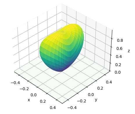
15. Forum für den lichttechnischen Nachwuchs
 Ilmenau, 04 – 06 Juni 2021

luminous intensity values in the rear half-space also influence the relative difference
here.

 Table 2: Features of Lambertian radiator with additive N(0, 0.01) noise

 Measurement
 origin [°] , ( , ) [°] [%] , [%] , [%]
 ( , , )

 (0, 0, 90) (0.02, -116.78) 65.84 17.70 75.42

 (0, 4, 90) (4.00, -90.03) 65.81 17.69 75.43

 (0, 11, 90) (11.00, -90.08) 65.83 17.70 75.29

In contrast to the form factor and the RAD, the maximum difference decreases. Since
the luminous intensity values must be greater than zero, the applied noise is no
longer without mean values. The maximum luminous intensity increases, the average
luminous intensity remains almost the same. This makes the maximum error smaller.

4.2 Narrow light sources
A bundled light source of the form 10 ( (0)) is now considered. The behavior of the
properties of LIDs shown in chapter 4.1 for an ideal Lambertian radiator should now
be evaluated for a simulated bundled light source.
Figure 3 shows the light distribution body of this light source. For the 10 -emitter, the
tests are also carried out for the ideal luminous intensity values and noisy values. The
results are summarized in tables 3 and 4.
The inclination angle of the radiation direction , is found just as well with the
bundled light source as with the Lambertian emitter. The azimuth angle of the
emission direction can be found more easily with the bundled light source. The clearly
narrower radiation characteristic enables a better spatial allocation.
As expected, the form factor of the bundled source is significantly larger than that of
the Lambertian radiator. In addition, the relative difference and maximum error are

© 2021 by the authors. – Licensee Technische Universität llmenau, Deutschland. - 129 -

15. Forum für den lichttechnischen Nachwuchs
 Ilmenau, 04 – 06 Juni 2021

significantly higher compared to Lambert's radiators. However, all of the properties
listed are also independent of the squint of the virtual lamp in this case.

 Figure 3: Illustration of the LID of an ideal measured 10 -radiator

If the 10 -emitter points out of the optical axis, the inclination angle of the emission
direction is found to an accuracy of 0.05 °. In addition, as with the Lambertian radiator,
the form factor and the relative difference measure decrease with additive white noise.
The maximum difference decreases as well. Thus, the maximum difference shows a
different behavior for 1 - and 10 -emitters.

 Table 3: Features of the LID of an ideal measured 10 -radiator

 Measurement
 , 
 origin [°] , ( , ) [°] [%] , [%]
 [%]
 ( , , )

 (0, 0, 90) (0.00, 160.73) 91.04 26.35 95.45

 (0, 4, 90) (4.00, -90.00) 91.06 26.36 95.44

 (0, 11, 90) (11.00, -90.00) 91.15 26.38 95.44

© 2021 by the authors. – Licensee Technische Universität llmenau, Deutschland. - 130 -

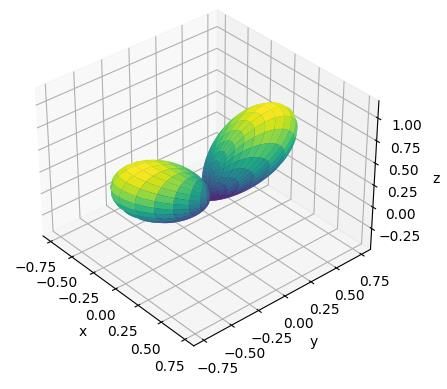
15. Forum für den lichttechnischen Nachwuchs
 Ilmenau, 04 – 06 Juni 2021

 Table 4: Features of a 10 -radiator with additive N(0, 0.01)-noise

 Measurement
 , 
 origin [°] , ( , ) [°] [%] , [%]
 [%]
 ( , , )

 (0, 0, 90) (0.08, -123.27) 89.62 26.10 95.26

 (0, 4, 90) (4.08, -89.94) 89.63 26.11 95.24

 (0, 11, 90) (11.00, -89.62) 89.65 26.11 95.23

4.3 Multi lobe light sources
In further investigations it should be shown that the proposed properties also apply to
light distributions consisting of two lobes. To do this, a luminaire is first simulated which
emits into the rear half-space with a 1 - and into the front half-space with a 10 -
characteristic. The light distribution body of this luminaire is shown in figure 4.

 Figure 4: Illustration of an ideal measured full space radiator

© 2021 by the authors. – Licensee Technische Universität llmenau, Deutschland. - 131 -

15. Forum für den lichttechnischen Nachwuchs
 Ilmenau, 04 – 06 Juni 2021

Table 5 shows the properties of the LID. The direction of radiation is found significantly
worse with this emitter than with the 1 - or the 10 -emitter. The form factor, as well
as the relative difference and maximum difference, also remain invariant to tilting in
this case.
Now white Gaussian noise is also added to this radiator. As in the previous
experiments, the direction of radiation is detected worse (see table 6). The form factor
becomes larger due to the noise.

 Table 5: Features of an ideal measured full space radiator

 Measurement
 , ( , )
 origin [°] [%] , [%] , [%]
 [°]
 ( , , )

 (0, 0, 90) (0.00, -118.77) 12.40 15.26 90.90

 (0, 4, 90) (3.99, -90.00) 12.42 15.26 90.89

 (0, 11, 90) (10.98, -90.00) 12.46 15.27 90.89

 Table 6: Features of a full space radiator with N(0, 0.01)-noise

 Measurement
 , ( , )
 origin [°] [%] , [%] , [%]
 [°]
 ( , , )

 (0, 0, 90) (0.69, 122.81) 12.81 15.15 91.00

 (0, 4, 90) (3.59, -92.92) 12.81 15.13 91.02

 (0, 11, 90) (10.76, -89.57) 12.88 15.15 90.96

This is due to the fact that more negative luminous intensity values are caused by the
noise in the rear half-space. The negative values come from the fact that the variance
of the noise is coupled to the maximum luminous intensity of the LID and is therefore
given by the 10 -radiator.
However, negative luminous intensity values are set to 0, which means that the noise
is no longer free of mean values. Therefore, the form factor increases with the noise.

© 2021 by the authors. – Licensee Technische Universität llmenau, Deutschland. - 132 -

15. Forum für den lichttechnischen Nachwuchs
 Ilmenau, 04 – 06 Juni 2021

With this light source, too, the relative difference and maximum difference behave
analogously to the Lambertian radiator.
Next, consider a radiator that consists of two 10 -lobes, which are inclined at
 = 0° and = 180° by 20 ° from the optical axis. The associated luminous intensity
distribution body is shown in Figure 5.
The properties for this light distribution are listed in table 7. The table shows that the
inclination angle of the radiation direction is found very precisely. If the measuring
surface is tilted by = 4° or = 11°, the angle of inclination is found precisely.
The form factor, the relative difference and the maximum difference are also invariant
to tilting for this LID. If the luminaire is additively superimposed with white noise, the
direction of radiation is found with an accuracy of 0.02 ° (table 8).

 Figure 5: Illustration of a LID consisting of two narrow lobes each squinting 20° from the optical axis

For the last experiment, the 10 -lobes of the radiator are now tilted 50 ° from the
optical axis. The associated luminous intensity distribution body is shown in figure 6.
With the simulation of this luminaire, the influence of a broad radiation and an
ambiguous main radiation direction on the characteristics of a LID presented in this
paper is to be examined.
The associated results can be found in table 9. With this LID, the direction of
radiation can be determined very precisely.

© 2021 by the authors. – Licensee Technische Universität llmenau, Deutschland. - 133 -

15. Forum für den lichttechnischen Nachwuchs
 Ilmenau, 04 – 06 Juni 2021

As a result of the wide radiation, the azimuth angle of the radiation can now also be
determined very precisely in addition to the angle of inclination. The angle of
inclination can be determined with an accuracy of 0.02°, the azimuth angle with an
accuracy of 0.05°. The form factor, the relative difference and the maximum
difference are also invariant to tilting of this LID.

 Table 7: Features of an ideal measured radiator consisting of two narrow lobes each squinting 20° from the
 optical axis

 Measurement
 , ( , )
 origin [°] [%] , [%] , [%]
 [°]
 ( , , )

 (0, 0, 90) (0.00, -37.34) 85.82 24.73 91.73

 (0, 4, 90) (4.02, -90.00) 85.82 24.73 91.74

 (0, 11, 90) (11.05, -90.00) 85.82 24.73 91.75

 Table 8: Features of a LID consisting of two narrow lobes each squinting 20° from the optical axis with
 N(0, 0.01)-noise

 Measurement
 origin [°] , ( , ) [°] [%] , [%] , [%]
 ( , , )

 (0, 0, 90) (0.01, -26.70) 84.82 24.54 91.57

 (0, 4, 90) (4.03, -89.71) 84.79 24.54 91.62

 (0, 11, 90) (11.09, -90.11) 84.91 24.55 91.63

If this LID is superimposed with white Gaussian noise, the direction of radiation is
significantly more robust compared to the previous light distributions. The form factor,
the relative difference and the maximum difference measure show the same behavior
in the case of noise as with the 1 - and the 10 -emitter.

© 2021 by the authors. – Licensee Technische Universität llmenau, Deutschland. - 134 -

15. Forum für den lichttechnischen Nachwuchs
 Ilmenau, 04 – 06 Juni 2021

 Figure 6: Illustration of a LID consisting of two narrow lobes each squinting 50° from the optical axis

 Table 9: Features of an ideal measured radiator consisting of two narrow lobes each squinting 50° from the
 optical axis

 Measurement
 , ( , )
 origin [°] [%] , [%] , [%]
 [°]
 ( , , )

 (0, 0, 90) (0.00, -54.88) 58.92 22.77 90.91

 (0, 4, 90) (4.01, -90.00) 58.92 22.77 90.90

 (0, 11, 90) (11.02, -90.00) 58.91 22.76 90.90

© 2021 by the authors. – Licensee Technische Universität llmenau, Deutschland. - 135 -

15. Forum für den lichttechnischen Nachwuchs
 Ilmenau, 04 – 06 Juni 2021

4.4 Discussion
In all cases, the calculated emitting direction follows the tilting of the initial LID. The
error of the emitting direction is smaller than the angular resolution ( = = 2.5°).
However, the quality of the calculated emitting direction strongly depends on the
magnitude of the form factor. If the form factor is close to zero, the radiation direction
depends on noise.
The relative difference and the maximum difference of ideal measured LIDs are
constant for tilting with less than 0.1% error. With noise, the values of the proposed
features differ to the features of ideal measured LIDs.
This means that the properties can be used to compare two identical light distributions.
On the basis of the properties presented, noise and squinting of the LID can be
distinguished after the measurement.

 Table 10: Features of a LID consisting of two narrow lobes each squinting 50° from the optical axis with
 N(0, 0.01)-noise

 Measurement
 , ( , )
 origin [°] [%] , [%] , [%]
 [°]
 ( , , )

 (0, 0, 90) (0.07, -87.99) 58.02 22.62 90.72

 (0, 4, 90) (4.10, -89.88) 58.06 22.60 90.80

 (0, 11, 90) (10.98, -90.06) 57.94 22.59 90.79

© 2021 by the authors. – Licensee Technische Universität llmenau, Deutschland. - 136 -

15. Forum für den lichttechnischen Nachwuchs
 Ilmenau, 04 – 06 Juni 2021

5 Summary and future work
For the comparison of LIDs, a feature-based approach was chosen in this paper in
order to differ between systematic errors and stochastic uncertainties of the measured
LIDs.
The presented method was evaluated on synthetic LIDs. The synthetic LIDs are
manipulated to simulate systematic errors. In our approach synthetic LIDs are rotated.
In order to find those rotations a mathematical formulation for the emitting direction is
proposed. Moreover, rotation invariant features were presented.
The features presented are sensitive to noise and are therefore suitable for
distinguishing between systematic errors, namely rotation errors, and stochastic
uncertainties.
In a new version, the generator is supposed to simulate measurement errors due to
incorrect positioning of the luminaire during the measurement. Incorrect calibration of
the measurement distance and the resulting errors when calculating the luminous
intensities should be considered.
Furthermore, there should be more investigation about the behavior of features
regarding systematic errors and different distributions and magnitudes of noise.
In addition, it is possible to calculate the homogeneity and isotropy of LIDs based on
histograms of luminous intensities. Histogram-based approaches are more robust and
more general compared to single values.

© 2021 by the authors. – Licensee Technische Universität llmenau, Deutschland. - 137 -

15. Forum für den lichttechnischen Nachwuchs
 Ilmenau, 04 – 06 Juni 2021

Literatur

[1] ASJ Bergen, „A practical method of comparing luminous intensity distributions, “
 Lighting, Research & Technology, Vol. 44, Issue 1, pp. 27-36, 2012.

[2] F Gassmann, U. Krueger, T. Bergen, F. Schmidt, „Comparison of luminous
 intensity distributions, “ Lighting, Research & Technology, Vol. 49, Issue 1, pp.
 62-83, 2017.

[3] N. Haferkemper, C. Vandahl, A. Stockmar, B. Hölzemann, „LVK-GENERATOR -
 Software zur Erzeugung virtueller Lichtstärkeverteilungen,“ Deutsche
 Lichttechnische Gesellschaft e.V. (LiTG), ISBN 978-3-927787-55-1, 1. Auflage
 2016.

[4] M. Katona, K. Trampert, C. Neumann, „System analysis of ILMD-based LID
 measurements using Monte Carlo simulation,“ eingereicht bei 14th International
 Conference on New Developments and Applications in Optical Radiometry
 (NEWRAD 2021), 2021.

[5] M. Katona, K. Trampert, C. Neumann, „Fehlerabschätzung der Fernfeldannahme
 bei LVK-Messungen mittels Nahfelddaten,“ LICHT2021, 2021.

© 2021 by the authors. – Licensee Technische Universität llmenau, Deutschland. - 138 -