Uncertainties, stochastic and deterministic components in radiation modelling - COSMO model

Uncertainties, stochastic and
 deterministic components in
 radiation modelling

Sophia Schäfer 1, Martin Köhler1, Robin Hogan2,3, Maike Ahlgrimm1,
 Daniel Rieger1, Axel Seifert1, Alberto de Lozar 1, Günther Zängl1
 1 Deutscher Wetterdienst, 2 ECMWF, 3 University of Reading

Radiation: From photons …
 Shortwave
 • Visible / thermal photons
 interact with surface,
 Longwave
 atmospheric gases, aerosol,
 cloud water or ice particles
 • Described by electromagnetic
 Maxwell equations and
 quantum mechanics, BUT can‘t
 treat every photon and
 atmospheric particle!
 • Have to capture bulk effect of
Photo R. Hogan each component

 2

… to global radiation budget, weather and climate

 Fluxes in W/m²
 Stephens et al. 2012

Radiation controls energy balance of Earth system, energy distribution throughout the
atmosphere → drives weather and climate dynamics and physics
Anthropogenic climate change: 2 W/m² global radiation imbalance (Myhre et al. 2013)
 3

Radiation scheme in global model
 Radiation model
From atmosphere model:
 • Optical property parametrisation for each
 – temperature, humidity component: optical depth, single scattering
 – gases, aerosol, surface properties albedo, asymmetry factor
 (usually climatology)
 • Radiation solver calculates radiative fluxes,
 – Clouds: cloud fraction, liquid & ice
 water content, effective particle • From fluxes: heating rates
 radius

• Radiative fluxes depend on atmosphere input + radiation scheme parametrisations to
 make calculation practical; for efficiency use coarser radiation grid, long radiation timestep
• Model tuned to top-of-atmosphere radiative fluxes (directly observable)
• ICON: RRTM radiation scheme, from early 2021: ecRad (Hogan & Bozzo 2018)
 4

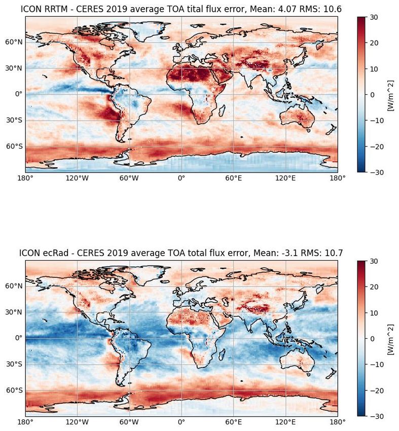
Impact of ecRad radiation scheme, / -Bugfix, Tuning
 Total TOA net radiation flux biases vs. CERES 2019 Upper air verification (2021, G. Zängl): Parallel routine
 Routine: / -Bug, tuned RRTM significant improvement in most variables and regions
 / -Bugfix, ecRad, tuning

 Total flux bias change:
 7 W/m² global

 Parallel routine: / -Bugfix, ecRad+LW scat.,
 new emissivity

New modular radiation scheme: ecRad (Hogan & Bozzo, 2018)
• Gas optics: • Solvers for radiative transfer equations:
  RRTMG (Iacono et al. 2008) – McICA (Pincus et al. 2005),
  ecCKD (Hogan 2010 JAS, under Tripleclouds (Shonk & Hogan,
 development): Fewer spectral 2008) or SPARTACUS (Schäfer et
 intervals but similar precision al. 2016, Hogan et al. 2016)
 – SPARTACUS makes ecRad the only
• Aerosol optics: variable species number global radiation scheme that can
 and properties (set at run-time) do sub-grid 3D radiative effects
• Cloud optics: – Longwave scattering optional
  liquid: SOCRATES (MetOffice), – Can configure cloud overlap
 Slingo (1989)
 – Cloud inhomogeneity: can
  ice: Fu 1996, 1998 (default) , configure width and shape of PDF
 Yi et al. 2013 or Baran et al. 2014

• Surface (under development) Implementation in ICON:
 Consistent treatment of urban and forest D. Rieger, M. Köhler,
 canopies R. J. Hogan, S. A. K. Schäfer,
 A. Seifert, A. de Lozar and
 Modular: can vary optics components and G.Zängl (2019): ecRad in
 solver individually to determine uncertainties ICON – Implementation
 Overview, Reports on ICON

Radiation spectra and atmospheric gases
• Molecules have different modes
 (vibration, rotation)
 Water molecule:
 vibration

 rotation

 commons.wikimedia.org
• Absorption / emission: distinct
 lines at energy steps → need high
 spectral resolution
• Divide spectrum into bands with
 similar Planck function, sub-divide
 and re-order into g-points to
 approximate gas absorption
• ICON uses RRTMG (Mlawer et al.
 1997, Iacono et al. 2008): 14 bands
 in shortwave, 16 in longwave,
 ~200 g-points
 7
 commons.wikimedia.org

Longwave
 Gas model uncertainty
• CKDMIP project: evaluate against
 exact line-by-line calculations for
 50 profiles (Hogan and Matricardi
 2020, https://confluence.ecmwf.int/
 display/CKDMIP/)
• Shortwave: outdated band
 spectrum of solar incoming flux in
 RRTMG v.3.9 (2013) (blue lines)
 Scaling solar spectrum to
 Coddington et al. (2016) data
 (more visible, less UV) reduces
 ecRad-RRTMG biases (red lines) to
 0 to 2 W/m²
 Shortwave
• New whole-spectrum gas model
 ecCKD (R. Hogan): Up to 60% faster,
 lower biases, can be optimised for
 each application (weather,
 climate,…), could include several
 vesions in ensemble
 Hogan and Matricardi
 8
 (2020)

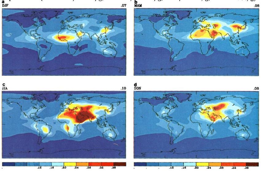
Gas, Aerosol and surface input property uncertainty
• Gases: mixing ratio constant /profile
 some (little) variability missing Winter Spring

• Aerosols: monthly climatology of optical
 properties in external parameter file
 (default: Tegen et al. 1997); Alternatives: Summer Autumn
 aerosol advection, ICON-ART: advection,
 chemistry + optical properties
 Variability missing: in IFS represented in SPP
 (Lang et al 2021); ICON uncertainty
 estimation in progress (PP CAIIR)
 Total aerosol optical depth in Tegen et al. (1997) climatology

• Surface albedo and emissivity: monthly climatology, modified for soil moisture, snow, sea ice
 Surface property uncertainty: ~2W/m² globally

Radiation solver: Two-stream equations
• Simplifications (→ systematic model uncertainties)
 – ignore phase, polarisation
 – only treat up-/downward flux instead of radiances in all directions (2 streams)
 – scattering phase function described by one parameter: asymmetry factor g
 – cloudy and homogeneous clear region of gridbox (strong effects of sub-grid clouds)
• Treat direct solar radiation separately; Diffuse radiation: assume solar zenith
 angle θdiff to approximate integral over angles
 Loss due to Extinction Gain from Scattering Internal source
 θdiff θdiff ↓
 clear ↓ ↑ ↓
 
 = βext −γ1,clear clear + γ2,clear clear + clear
 ↑clear ↑ ↓ ↑
 - 
 = βext −γ1,clear clear + γ2,clear clear + clear
 θdiff θdiff

• Multi-layer: need to know how clouds overlap vertically, also horizontal inhomogeneity
 Clouds largest uncertainty 10

Sub-grid cloud geometry in radiation solvers
 All solvers for global models simplify by treating only vertical dimension explicitly.
 Deterministic: Stochastic:
 McICA (ecRad): draw random
Two-stream solver (e.g. RRTM in Tripleclouds/SPARTACUS (ecRad): clouds in sub-columns for overlap
ICON): solve in cloudy / clear similar; 3 regions: clear, thin + inhomogeneity; distribute
regions, partition at layer cloud, thick cloud → cloud spectral intervals in 1 sub-column
boundaries according to overlap inhomogeneity each → fast, random noise

 Plots adapted from R. Hogan

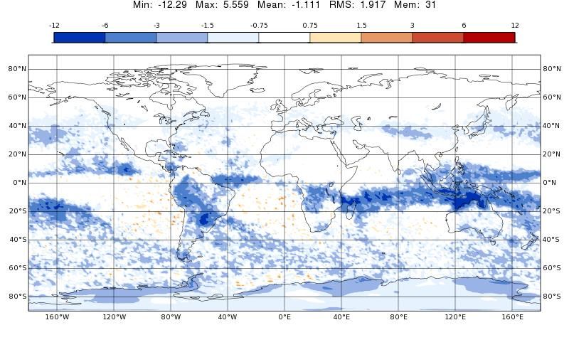
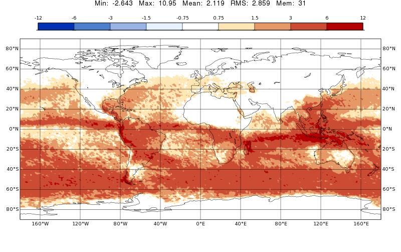
Solver uncertainty in ICON+ecRad: Tripleclouds-McICA (Jan 2018, 24h runs)
 T T SW tendency T LW tendency
 -0.4 -0.2 -0.1 -0.05 -0.025 0.025 0.05 0.1 0.2 0.4 K -0.04 -0.02 -0.01-0.005 -0.0025 0.0025 0.005 0.01 0.02 0.04 K/d -0.4 -0.2 -0.1 -0.05 -0.025 0.025 0.05 0.1 0.2 0.4 K/d

 SW TOA flux LW TOA flux
 Sytematic differences -12 -6 -3 -1.5 -0.75 0.75 1.5 3 6 12 W/m² -4 -2 -1 -0.5 -0.25 0.25 0.5 1 2 4 W/m²

 (more similar settings
 available) + random
 variability in McICA

Cloud vertical overlap
• For given cloud fraction in each layer, cloud overlap decides total cloud cover

 Adapted from Hogan & Illingworth 2000, QJRMS

• Based on observations (Hogan & Illingworth 2000): exponential-random overlap,
 decorrelation length ca. 2 km, small / BL cumulus: 100-600m (Neggers et al. 2011,
 Corbetta et al. 2015); Lang et al 2021: variation represented in SPP, mean 1 km;
• Realistically, decorrelation length should depend on situation / cloud type (Jing et
 al 2018, Sulak et al 2020, etc.)
 13

Cloud inhomogeneity: fractional standard deviation
• Reflectivity and longwave emissivity non-linear functions of optical depth /cloud water content

 • ICON RRTM reduces optical
 depth by factor 0.8 (COSMO 0.5)

 Plots by R. Hogan

• ecRad inhomogeneity parameters: cloud water distribution (gamma / lognormal PDF),
 standard deviation
 = , in IFS represented in SPP (Lang et al 2021)
 mean
 • Tripleclouds: two cloudy regions (equal size, preserve standard
 deviation of cloud water PDF)
 • McICA: random number ∈ [0,1] for each cloudy layer, correlated
 according to vertical inhomogeneity correlation; scale with cloud
 2*std. dev. water PDF value at this percentile
 Water content
 16% median
 14
 Adapted from Shonk & Hogan (2008)

Cloud fractional standard deviation (FSD) impact

 January 2019

 Change in SW TOA flux 2019: parametrised FSD vs FSD=1
 July 2019

 FSD parametrised by cloud type
 (Ahlgrimm and Forbes 2016, 2017)
 changes SW flux by 0.8 W/m² globally,
 Zonal mean LW by 0.1 W/m², synoptic noise
 parametrised →Need longer run for clearer signal
 in-cloud FSD

3D cloud effects
 b) Shortwave cloud side
 a) Shortwave cloud
 escape
 • Shortwave cloud side illumination
 side illumination increases cloud reflectivity, cloud side
 escape decreases cloud reflectivity
 • Longwave cloud side illumination and
 escape increase cloud warming effect
 c) Longwave cloud side d) Shortwave entrapment • Shortwave entrapment decreases
 illumination and escape cloud reflectivity
 • Similar effects at complex surfaces
 (trees / mountains / buildings)
 • Usually neglected, SPARTACUS solver in
 ecRad can treat them
 • Globally: total flux change 2 to 3 W/m²,
 warms Earth by ~1 , locally higher

 16

Cloud particle optics
 Cloud particles: ~ → Mie scattering:
 complex function of scattering angle

 • Simplify in 3 bulk optical parameters:
 optical depth , single scattering
 
 albedo = ,
 + 
 asymmetry parameter
 Scattering intensity ( , x) 1 2 
 Spherical particles, e.g. = ‫׬‬0 ‫׬‬0 cos θ 
 4 
 liquid droplets,
 Petty (2006) = forward – backward scattering

 • Optics look-up tables:
 , , (water content, particle size)
 17

Ice particle shape and effective radius
• Complex ice particle shapes → shape
 assumptions
• Fu ice optics (Fu 1996, 1998, default in
 ICON): hexagonal columns
• Alternatives in ecRad: Yi ice optics (Yi et al.
 2013), Baran ice optics (Baran et al. 2014):
 ice habit mixtures – precipitation neglected
 Plot by R. Hogan

 • Mixture of particle sizes in clouds
 Cloud ice • Parametrised input effective radius
 particle size = mean radius weighted by
 distributions
 (Delanoë et number, area, scattering efficiency of
 al 2005) each particle size
 • Definition needs to agree with optics
 18

Ice optics uncertainty in ICON+ecRad: Baran – Fu (Jan 2018, 24h runs)
 T T SW tendency T LW tendency
 -0.16 -0.08 -0.04 -0.02 -0.01 0.01 0.02 0.04 0.08 0.16 K -0.16 -0.08 -0.04 -0.02 -0.01 0.01 0.02 0.04 0.08 0.16 K/d -0.4 -0.2 -0.1 -0.05 -0.025 0.025 0.05 0.1 0.2 0.4 K/d

 SW TOA flux LW TOA flux
 Considerable uncertainty in
 ice optics assumptions: -12 -6 -3 -1.5 -0.75 0.75 1.5 3 6 12 W/m² -8 -4 -2 -1 -0.5 0.5 1 2 4 8 W/m²

 ~2W/m² globally, ~10W/m²
 locally, not well constrained
 Need effective radius
 consistent with ice optics
 shape assumptions

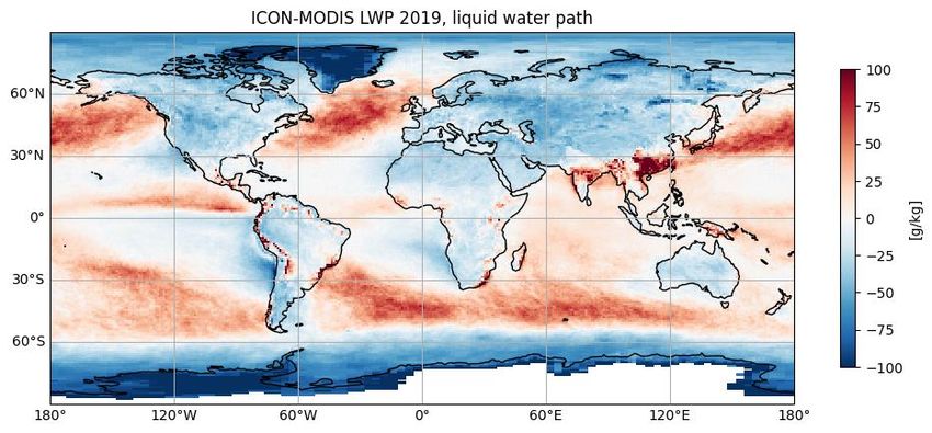
Cloud water content uncertainty
 Cloud liquid water
 path bias in ICON
 2019 compared to
 MODIS (left, 2019)
 and MAC-LWP
 (right, 2016-2019),
 by M. Ahlgrimm

• Radiation does not consider precipitation, except to
 add 10% of snow to cloud ice - neglects 50 %
 (liquid) to 80% (ice, Li et al. 2012) of total water
• Uncertainty in retrievals and microphysics
• Models tuned to TOA radiation balance → cloud
 water content between observed cloud and total
 water content
• Ongoing work (with R. Hogan, A. de Lozar, PP CAIIR):
 include general number of particle species + optics Cloud and total ice water path in ECHAM6.3
 for large particles → precipitation in ecRad and CALIPSO-GOCCP (Dietlicher et al. 2019)

Cloud particle size parametrisation

• Currently: ice effective radius for Microphysics

 radiation independent of and
 inconsistent with microphysics Radiation
 (liquid easier: spherical droplets)
 reff ( m) reff ( m) reff ( m)

• Ongoing work (Alberto de Lozar): Frequency Frequency Frequency
 effective radius for radiation
 consistent with 1-moment- or
 2-moment-microphysics

• Could use stochastic
 microphysics for uncertainty (in
 IFS: SPP, Lang et al 2021)
 Plots by A. de Lozar

Cloud feedback: ecRad versus RRTM in ICON single column model
 0.0002
 height RRTM ecRad
 0

Longwave heating rate
 -0.0002

 -0.0004 K/s

 -0.0006

 More
 -0.0008
 Heating rate realistic
 oscillation bug -0.001
 time
 time
 height

 Cloud water

Summary and Outlook
• Largest uncertainty in both radiation model and input: Clouds
• ecRad improves ICON, can vary optics parametrisations, solver, cloud overlap and
 inhomogeneity treatment → can estimate and include parameter and
 parametrisation uncertainty; stochastic treatment of cloud geometry
• Several components have uncertainties of 1 to 10 W/m²

Next steps:
• General number of hydrometeor species → include snow, graupel, rain in radiation,
 evaluate and adjust water content in model
• Vary overlap and vertical decorrelation length parametrisation
• More consistent particle size and shape treatment
• Ensemble including ecRad parametrisation range?
• Ongoing model evaluation for all applications, incl. feedbacks

 Thank you for your attention!
 Contact: sophia.schaefer@dwd.de 23

Gas optics model: bands

• Divide spectrum into
 bands where Planck

 Planck function
 function is similar

• ICON uses RRTMG
 (Mlawer et al. 1997,
 Water vapour spectrum

 Iacono et al. 2008):
 14 bands in shortwave,
 16 in longwave

 24
 Plot by R. Hogan

Gas optics: g-points / correlated-k-method
• In each band:
 – Approximate Planck

 Planck function
 function
 – Re-order by gas
 absorption,
 approximate in 6-21
 g-points
 (Lacis, Oinas 1991)
 Water vapour spectrum

• RRTMG: ~200 g-points

• Could reduce cost by re-
 ordering full spectrum
 (Hogan 2010 JAS)
 25
 Plot by R. Hogan

Alternative gas optics: full-spectrum correlated-k-method
• Re-order whole spectrum,
 average Planck emission

 Planck function
 for wavelengths in each
 g-point (Hogan 2010, JAS)
• With 40 g-points: cheaper,
 more precise that RRTMG
 - future in ICON?

 Water vapour spectrum

 ecRad longwave heating rate error on 50 test 26
 profiles, RRTMG and ecCKD gas optics Plots by R. Hogan

ecRad in ICON with new solar spectrum

• Scaling improves agreement with
 line-by-line calculations, removes
 spurious stratospheric heating
• With new spectral scaling, ecRad
 improves ICON results in both
 troposphere and stratosphere vs.
 RRTM radiation scheme
• RRTM also uses RRTMG gas
 model – less sensitive

Gas model /spectrum uncertainty
up to 2 W/m², not now represented
Future ecCKD gas model: less uncertainty, cheaper,
could use different versions in ensemble

Global total 3D cloud effects
 Total 3D effect on climate
 • Global fluxes (net down,
 surface):
 Longwave +1.6 Wm−2,
 Shortwave +0.8 Wm−2,
 Total +2.4 Wm−2
 • Temperature increases by
 around 1K.
 • Depends on entrapment and
 cloud geometry (Schäfer et
 al., in prep.)

 Mean 3D effect on temperature in four
 1-year simulations with coupled ocean,
 with minimum (top) / calculated
 Coupled (middle) / maximum (base) entrapment.

Vertical cloud overlap uncertainty
 Neggers, Heus, Siebesma, 2011 Decorrelation length scale: Hogan, Illingworth, 2000
 220m Decorrelation length scale:
 cc proj 1600m

 Layer thickness [m]

 Chilbolton, radar, dz=360m, dt=1h

 cfmean
 cfmean /cc proj
 LES simulation of BOMEX cumulus (dz=10m)

Corbetta, Orlandi, Heus, Neggers, Crewell, 2015 100-600m

 Jülich cases LES forced by ECMWF (dz=40m)

Scattering by particles
 
 • Scattering intensity at scattering angle 
 2 
 depends on size parameter = : ratio
 
 of particle radius and wavelength 
 • ≫ : Geometric optics
 • ≪ : Rayleigh scattering: particle acts as
 electric dipole, scattering intensity
 3
 = (1 + cos 2) 
 4

 • Rayleigh scattering efficiency Qs ∝ 4
 Petty (2006)
 (measures scattering per particle area)

 30

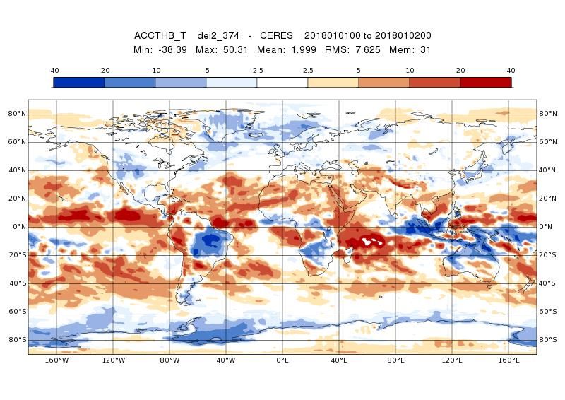
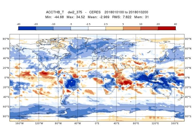
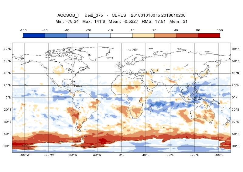
Evaluation (CERES): RRTM and first ecRad, 24h forecasts, Jan. 2018
 TOA solar vs. CERES TOA thermal vs. CERES
 bias: 0.92 W/m2 bias: 1.99 W/m2
 -160 -80 -40 -20 -10 10 20 40 80 160 W/m² -40 -20 -10 -5 -2.5 2.5 5 10 20 40 W/m²

 RRTM

 bias: -0.52 W/m2 bias: -2.99 W/m2
 -160 -80 -40 -20 -10 10 20 40 80 160 W/m² -40 -20 -10 -5 -2.5 2.5 5 10 20 40 W/m²

 ecRad
 first version
 - not tuned

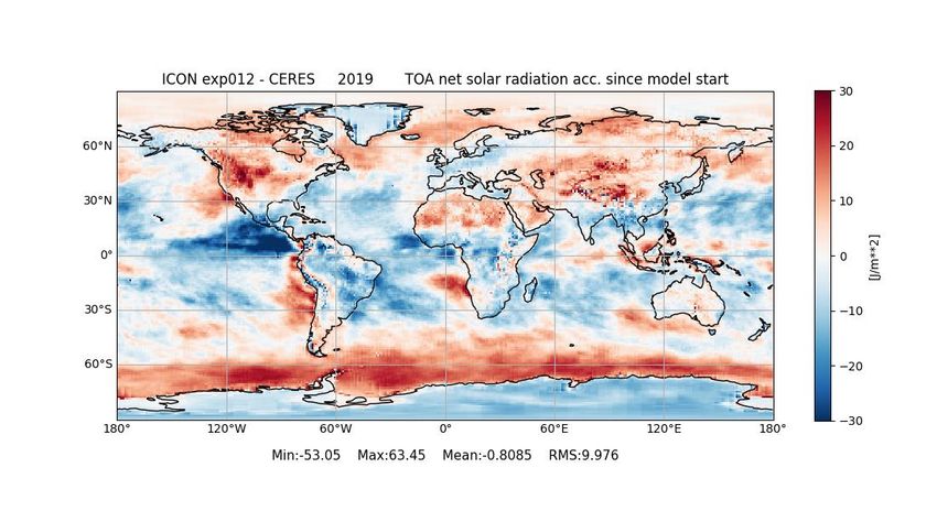
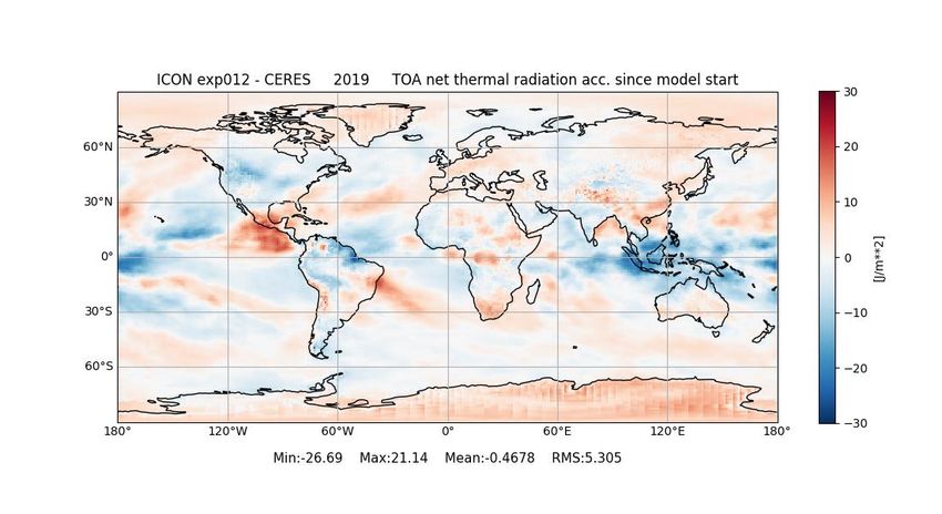
Evaluation vs. CERES 2019 all year: Energy bugfix + ecRad + LW scat.
 Energy bugfix+ ecRad
 TOA solar vs. CERES bias: -0.81 W/m2 + cloud LW scattering TOA thermal vs. CERES bias: -0.47 W/m2

 Resolution R2B6, Δ ≈40 km