Observation uncertainty in data assimilation
←
→
Page content transcription
If your browser does not render page correctly, please read the page content below
Observation uncertainty in data assimilation

                  Sarah L. Dance
email: s.l.dance@reading.ac.uk twitter: @DrSarahDance

With thanks to collaborators at UoR, DWD and the Met Office including Elisabeth
Bauernschubert, John Eyre, Alison Fowler, Graeme Kelly, Amos Lawless, Stefano
Migliorini, Andrew Mirza, Nancy Nichols, Roland Potthast, Gabriel Rooney, David
 Simonin, Fiona Smith, Laura Stewart, Ed Stone, Jemima Tabeart, Jo Waller....
Outline

What are observation errors?

Why estimate observation uncertainty?

How can we estimate observation uncertainty?

What are the pitfalls?

What are the possibilities?

Conclusions

 2 of 32
What are observation errors?
In data assimilation, we consider
the observation equation

            y = H(x) + ε.

We assume ε is unbiased,
E(ε) = 0, and has covariance R
such that

            Rij = E(εi εj ).

  3 of 32
Where do observation errors come from?
The error vector, ε, contains errors from four main sources: Janjić
et al (2017)

 Instrument noise                     Observation pre-processing

 Observation operator error           Scale mis-match

 4 of 32
Why do we want to estimate observation
uncertainty?
• Only use 5% of some obs types due to thinning

5 of 32

Why do we want to estimate observation
uncertainty?
• Only use 5% of some obs types due to thinning

• Improve analysis accuracy and forecast skill (e.g., Stewart et al.
  2013; Weston et al., 2014)

5 of 32
Why do we want to estimate observation
uncertainty?
• Only use 5% of some obs types due to thinning

• Improve analysis accuracy and forecast skill (e.g., Stewart et al.
  2013; Weston et al., 2014)
• Changes to scales of observation information content in
  analysis depending on both the prior and observation error
  correlations (Fowler et al, 2018)

5 of 32
Estimating observation uncertainty

• In DA, observation uncertainty depends on YOUR observation
  operator, model resolution etc and is state dependent (Waller et
  al., 2014; Janjić et al, 2018)
• Approximations are still useful and can give improved forecast
  skill (Healy and White, 2005; Stewart et al, 2013)

6 of 32
How can we estimate observation uncertainty?

• Error inventory/Metrological approach

7 of 32
How can we estimate observation uncertainty?

• Error inventory/Metrological approach
• Collocation with other observations (but rep. error?)

7 of 32
How can we estimate observation uncertainty?

• Error inventory/Metrological approach
• Collocation with other observations (but rep. error?)
• Diagnosis from assimilation (review by Tandeo et al, 2020)
  ◦ Moment based methods (e.g., using innovation and residual
    statistics, Desroziers et al, 2005)

7 of 32
How can we estimate observation uncertainty?
• Error inventory/Metrological approach
• Collocation with other observations (but rep. error?)
• Diagnosis from assimilation (review by Tandeo et al, 2020)
◦ Moment based methods (e.g., using innovation and residual
statistics, Desroziers et al, 2005)
◦ Likelihood based methods (e.g., expectation maximization, Pulido
et al, 2018)
7 of 32DBCP diagnostic (Desroziers et al 2005)
• Easy to compute from
Early IASI example (Stewart et al.,
standard innovations and 2009, 2014.)
analysis residuals
• Proven useful in NWP
• Non-symmetric structure
8 of 32DBCP diagnostic, Desroziers et al., (2005)
Use the background innovations and analysis residuals:
dob = y − H(xb ),
9 of 32DBCP diagnostic, Desroziers et al., (2005)
Use the background innovations and analysis residuals:
dob = y − H(xb ),
doa = y − H(xa ).
9 of 32DBCP diagnostic, Desroziers et al., (2005)
Use the background innovations and analysis residuals:
dob = y − H(xb ),
doa = y − H(xa ).
Taking the statistical expectation, and after some calculations...
T −1
E[doa dob ] = R(H
e BHe T + R)
e (HBHT + R) = Re ,
where
• Re is the estimated observation error covariance matrix
• B and R are the exact background and observation covariance
matrices.
• R
e and B e are the assumed statistics used in the assimilation.
9 of 32DBCP diagnostic, Desroziers et al., (2005)
Use the background innovations and analysis residuals:
dob = y − H(xb ),
doa = y − H(xa ).
Taking the statistical expectation, and after some calculations...
T −1
E[doa dob ] = R(H
e BHe T + R)
e (HBHT + R) = Re ,
where
• Re is the estimated observation error covariance matrix
• B and R are the exact background and observation covariance
matrices.
• Re and Be are the assumed statistics used in the assimilation.
If R = R and B
e e = B, then
T
E[doa dob ] = R.
9 of 32What are the pitfalls? 10 of 32
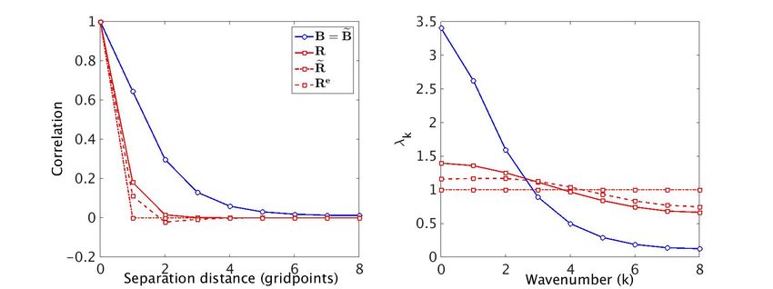
Sensitivity to Assumed Statistics (Waller et al,
2016 QJ)
T −1
E[doa dob ] = R(H
e BHe T + R)
e (HBHT + R) = Re ,
Example: True background error stats, B
e = B; diagonal R
e
Re has an underestimated variance and correlation lengthscale,
but is a better approximation than R.
e
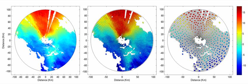
11 of 32Doppler radar winds and Met Office UKV 12 of 32
Horizontal Correlations, sensitivity to B
                                        e
Waller et al. (2016) MWR

• Increasing variance and lengthscale in B
                                         e reduces variance and
  lengthscale in diagnosed Re .
• Consistent with Waller et al (2016) QJ theory.
13 of 32
DBCP and Local DA (Waller et al, 2017)
• DBCP does not always give the right answers. Must only
calculate with the right set of points.
Regions of observation influence
The region of influence of an
observation is the set of analysis states
that are updated in the assimilation
using the observation.
Grid points (pluses) and observations
(dots), with observations coloured with
corresponding regions of observation
influence (shaded coloured circles).
14 of 32DBCP and Local DA Cont(Waller et al, 2017) The domain of dependence of an observation yi is the set of elements of the model state that are used to calculate the model equivalent of yi Example: The coloured squares around grid points select the points that would be utilized by the observation operator for the observation of the corresponding colour. The correlation between the errors of observations yi and yj can be estimated using the DBCP diagnostic only if the domain of de- pendence for observation yi lies within the region of influence of observation yj . 15 of 32
What are the possibilities?

16 of 32
Comparison of approaches (Mirza et al, 2021)
• Mode-S EHS temperatures - errors from lack of precision in
   Mach number
• Diagnosed std (black-dashed-squares) compare well with
   metrological estimates (red diamonds)

                           14

                           12
                                                                                      Estimates of observation error:
                           10
                                                                                      Assumed
           Pressure Altitude (km)

                                                                                      Empirical
                                    8                                                 Diagnosed

                                    6

                                    4

                                    2

                                    0
                                        0        1               2                3                    4                5

                                -2
                                            Observation Standard Deviation - Mach Temperature Reports (K)
17 of 32
Identifying sources of error - Examples
Waller et al (2016) Rem. sens. Bauernschubert et al (2019)
SEVIRI interchannel error covari- Doppler radar wind error std
ances over different subdomains
Land-sea QC issue Radars 10169 and 10204 contam-
inated by wind turbines and ship
tracks
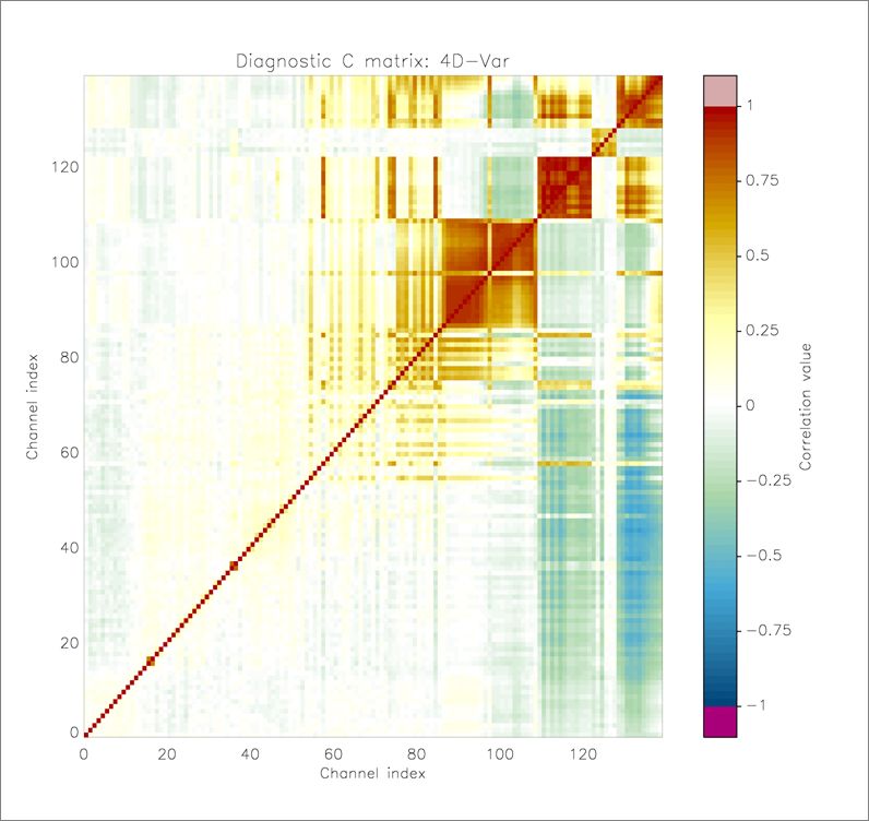
18 of 32Using diagnosed covariances in operational
systems
Problems: Diagnosed
covariances typically
• Not symmetric
• Not positive definite
• Variances too small
• Ill-conditioned
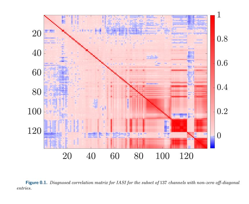
Diagnosed interchannel observation error correlations for
IASI (for the Met Office global model)
Can prevent convergence of variational minimization (Weston et
al. 2014)
19 of 32Convergence of minimization
The sensitivity and accuracy of the solution of the minimization
depend on the condition number of the Hessian
λmax (S)
κ(S) = ,
λmin (S)
where λ denotes the eigenvalue and the Hessian is
S = B−1 + HT R−1 H.
Tabeart et al. (2018) showed that κ(S) increases with λmin (R).
Tabeart et al. (2021) showed similar results with pre-conditioned
form (control var transform).
20 of 32Reconditioning R To improve the conditioning of R (and S ) we alter the eigenstructure of R so as to obtain a specified condition number for the modified covariance matrix by e.g., • Ridge regression - add constant to all diagonal elements. • Eigenvalue modification: increase the smallest eigenvalues of R to a threshold value that ensures the desired condition number, keeping the rest unchanged. 21 of 32
Reconditioning results with IASI inter-channel
error matrix (Tabeart et al, 2020)

• Ridge regression method increases standard deviations more
   than minimum eigenvalue method
• Ridge regression method decreases correlations, but minimum
   eigenvalue method has non-uniform behaviour
22 of 32
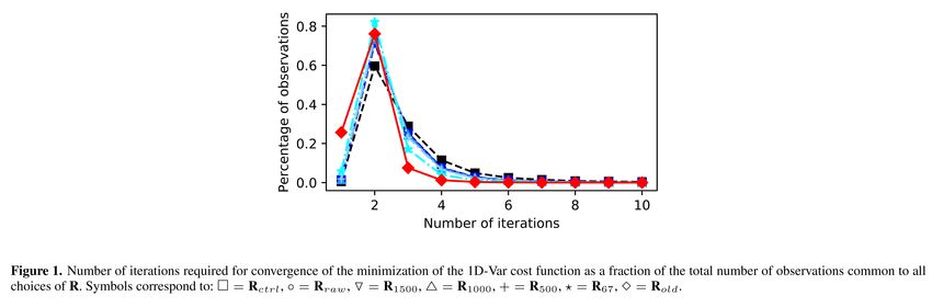
Experiments with Ridge Regression in Met Office
1D-Var (Tabeart et al. 2020)

• Reconditioning increases convergence speed

23 of 32
Experiments with Ridge Regression in Met Office
1D-Var (Tabeart et al. 2020)

• Reconditioning increases convergence speed
• Lots of examples of improved forecast skill from taking account
   of interchannel error covariances (Met Office, ECMWF, NRL,
   ECCC, NASA, NCEP, Meteo France...)
23 of 32
Spatial correlations

We need to be able to compute
the matrix-vector product

             R−1 v.

This might require expensive
communication between
processors.

  24 of 32
Doppler radar wind assimilation (Simonin et al, 2019)
• Assume only horizontal correlations within a family
• R is derived on-the-fly (different observations each assimilation)
• Correlation matrix is determined by calculating the distance
between each pair of observations in the family
−Dij
Cij = exp
Lr
• Lengthscale determined by fitting to diagnosed horizontal
correlations
25 of 32Experiments Three experiments run for 20 days (3 hourly cycling 3D-Var, UKV 1.5km model) Control: 6km thinning with diagonal R (∼ 2000 radar obs per cycle) Corr-R-6km: 6km thinning with correlated R (∼ 2000 radar obs per cycle) Corr-R-3km: 6km thinning with correlated R (∼ 8000 radar obs per cycle) 26 of 32
Results
• No significant difference in iteration count or wall-clock time

27 of 32
Results
• No significant difference in iteration count or wall-clock time
• Corr-R-3km increments are smaller scale and smaller
   magnitude

27 of 32
Results
• No significant difference in iteration count or wall-clock time
• Corr-R-3km increments are smaller scale and smaller
   magnitude
• Parameters for experiments have not been tuned, but most
   O-Bs show a small benefit from the introduction of correlations.
                       σO−B,exp
                                  − 1[%]
                        σO−B,ctrl

27 of 32
O-B Forecast skill cont Work 28 of 32 underway to implement in 4D-Var.
Conclusions
• It is important to be able to account for observation error
   correlations
    ◦ Avoid thinning (high resolution forecasting)
    ◦ Improved forecast skill score

29 of 32
Conclusions
• It is important to be able to account for observation error
correlations
◦ Avoid thinning (high resolution forecasting)
◦ Improved forecast skill score
• First we need to estimate correlations
◦ Desroziers et al (2005) diagnostic can be used with caution
◦ Can understand sensitivity to the assumed stats in the assimilation
(Waller et al. 2016a)
◦ Can help us to understand sources of correlations (e.g., Waller et
al 2016b)
29 of 32Conclusions
• It is important to be able to account for observation error
correlations
◦ Avoid thinning (high resolution forecasting)
◦ Improved forecast skill score
• First we need to estimate correlations
◦ Desroziers et al (2005) diagnostic can be used with caution
◦ Can understand sensitivity to the assumed stats in the assimilation
(Waller et al. 2016a)
◦ Can help us to understand sources of correlations (e.g., Waller et
al 2016b)
• Then we need to be able to account for the errors in the
assimilation
◦ Sample matrices need reconditioning
◦ Appropriate software needs to be in place to deal efficiently with
full matrices
29 of 32References Page 1 Bathmann, K., 2018. Justification for estimating observation-error covariances with the Desroziers diagnostic. Quarterly Journal of the Royal Meteorological Society, 144(715), pp.1965-1974. G. Desroziers, L. Berre, B. Chapnik, and P. Poli. Diagnosis of observation, background and analysis-error statistics in observation space. Q.J.R. Meteorol. Soc., 131:3385-3396, 2005. Fowler, A. M., Dance, S. L. and Waller, J. A. (2018), On the interaction of observation and prior error correlations in data assimilation. Q.J.R. Meteorol. Soc., 144: 48-62. doi:10.1002/qj.3183 Healy, S.B. and White, A.A., 2005. Use of discrete Fourier transforms in the 1D-Var retrieval problem. Quarterly Journal of the Royal Meteorological Society: A journal of the atmospheric sciences, applied meteorology and physical oceanography, 131(605), pp.63-72. Janjić, T., Bormann, N., Bocquet, M., Carton, J.A., Cohn, S.E., Dance, S.L., Losa, S.N., Nichols, N.K., Potthast, R., Waller, J. and Weston, P., 2018. On the representation error in data assimilation. Quarterly Journal of the Royal Meteorological Society, 144(713), pp.1257-1278. Menard R. 2016. Error covariance estimation methods based on analysis residuals: theoretical foundation and convergence properties derived from simplified observation networks. Quarterly Journal of the Royal Meteorological Society 142: 257-273. Mirza, A.K., S.L. Dance, G. G. Rooney, D. Simonin, E. K. Stone and J. A. Waller Comparing diagnosed observation uncertainties with independent estimates: a case study using aircraft-based observations and a convection-permitting data assimilation system. Submitted Pulido, M., P. Tandeo, M. Bocquet, A. Carrassi, and M. Lucini, 2018: Stochastic parameterization identification using ensemble Kalman filtering combined with maximum likelihood methods. Tellus A: Dynamic Meteorology and Oceanography, 70 (1), 1442 099. L. M. Stewart, J. Cameron, S. L. Dance, S. English, J. R. Eyre, and N. K. Nichols. Observation error correlations in IASI radiance data. Technical report, University of Reading, 2009. Mathematics reports series, www.reading.ac.uk/web/FILES/maths/obs_error_IASI_radiance.pdf. L. M. Stewart, S. L. Dance, N. K. Nichols, J. R. Eyre, and J. Cameron. Estimating interchannel observation-error correlations for IASI radiance data in the Met Office system. Quarterly Journal of the Royal Meteorological Society, 140:1236-1244, 2014. doi: 10.1002/qj.2211. Stewart, L.M., Dance, S.L., Nichols, N.K. (2013) Data assimilation with correlated observation errors: experiments with a 1-D shallow water model, Tellus A doi: 10.3402/tellusa.v65i0.19546 30 of 32
References Page 2
J. M. Tabeart, S. L. Dance, S. A. Haben, A. S. Lawless, N. K. Nichols, and J. A. Waller (2018) The conditioning of least
   squares problems in variational data assimilation. Numerical Linear Algebra with Applications doi:10.1002/nla.2165
Jemima M. Tabeart Sarah L. Dance Amos S. Lawless Stefano Migliorini Nancy K. Nichols Fiona Smith and Joanne A.
   Waller (2020) The impact of using reconditioned correlated observation-error covariance matrices in the Met Office
   1D-Var system. QJR Meteorol Soc.146: 1372-1390. doi:10.1002/qj.3741
Jemima M. Tabeart, Sarah L. Dance, Amos S. Lawless, Nancy K. Nichols & Joanne A. Waller (2020) Improving the
   condition number of estimated covariance matrices, Tellus A: Dynamic Meteorology and Oceanography, 72:1, 1-19 doi:
   10.1080/16000870.2019.1696646
Jemima M. Tabeart, Sarah L. Dance, Amos S. Lawless, Nancy K. Nichols, Joanne A. Waller (2021) The conditioning of
   least squares problems in preconditioned variational data assimilation, submitted
Tandeo, P., P. Ailliot, M. Bocquet, A. Carrassi, T. Miyoshi, M. Pulido, and Y. Zhen, 2020: A Review of Innovation-Based
   Methods to Jointly Estimate Model and Observation Error Covariance Matrices in Ensemble Data Assimilation. Mon.
   Wea. Rev., 148, 3973-3994.
Waller JA, Ballard SP, Dance SL, Kelly G, Nichols NK, Simonin D. 2016. Diagnosing horizontal and inter-channel
   observation-error correlations for SEVIRI observations using observation-minus-background and
   observation-minus-analysis statistics. Remote Sens. 8: 581, doi: 10.3390/rs8070581.
Waller, J. A., Dance, S. L. and Nichols, N. K. (2016) Theoretical insight into diagnosing observation error correlations using
   observation-minus-background and observation-minus-analysis statistics. Q.J.R. Meteorol. Soc. doi: 10.1002/qj.2661
Waller, J. A., Simonin, D., Dance, S. L., Nichols, N. K. and Ballard, S. P. (2016b) Diagnosing observation error correlations
   for Doppler radar radial winds in the Met Office UKV model using observation-minus-background and
   observation-minus-analysis statistics. Monthly Weather Review. doi: 10.1175/MWR-D-15-0340.1
Waller, J.A., Dance, S.L. and Nichols, N.K. (2017), On diagnosing observation-error statistics with local ensemble data
   assimilation. Q.J.R. Meteorol. Soc., 143: 2677-2686. doi:10.1002/qj.3117
P. P. Weston, W. Bell, and J. R. Eyre. Accounting for correlated error in the assimilation of high-resolution sounder data.
   Quarterly Journal of the Royal Meteorological Society, 2014. doi: 10.1002/qj.2306.

   31 of 32
Iteration
• Iteration converges to the correct estimate only when assumed
  B
  e is correct (Menard, 2016; Bathmann, 2018)
• More often, the first iterate is used. Experience shows little
  difference between iterates.

Bathmann(2018) a) First iterate b) Sixth iterate correlation matrix
             for IASI with NCEP global system
32 of 32
You can also read