Supplement of Impacts of land use change and elevated CO2 on the interannual variations and seasonal cycles of gross primary productivity in China ...

Supplement of Earth Syst. Dynam., 11, 235–249, 2020
https://doi.org/10.5194/esd-11-235-2020-supplement
© Author(s) 2020. This work is distributed under
the Creative Commons Attribution 4.0 License.

Supplement of
Impacts of land use change and elevated CO2 on the interannual
variations and seasonal cycles of gross primary productivity in China
Binghao Jia et al.

Correspondence to: Binghao Jia (bhjia@mail.iap.ac.cn)

The copyright of individual parts of the supplement might differ from the CC BY 4.0 License.

1 S1 Models and data

 2 In this study, we used twelve terrestrial biosphere models (TBMs) that participated in the Multi-
 3 scale Synthesis and Terrestrial Model Intercomparison Project (MsTMIP) (Huntzinger et al., 2013;
 4 Wei et al., 2014a, 2014b) to investigate the effects of climate change, land use and land cover change
 5 (LULCC), and rising CO2 concentration on the temporal changes in GPP. These models are
 6 Community Land Model version 4 (CLM4; Shi et al., 2011; Mao et al., 2012), CLM4 with Variable
 7 Infiltration Capacity Runoff Parameterization (CLM4VIC; Lei et al., 2014), Dynamic Land Ecosystem
 8 Model (DLEM; Tian et al., 2011, 2012), Global Terrestrial Ecosystem Carbon model (GTEC; Ricciuto
 9 et al., 2011), Integrated Science Assessment Model (ISAM; Jain et al., 2013), Lund-Potsdam-Jena
10 Dynamic Global Vegetation Model, Swiss Federal Research Institute WSL modification (LPJ-wsl;
11 Sitch et al., 2003), Organizing Carbon and Hydrology in Dynamic Ecosystems (ORCHIDEE-LSCE;
12 Krinner et al., 2005), Simple Biosphere version 3 by Jet Propulsion Laboratory (SiB3-JPL; Baker et
13 al., 2008), SiB3 with Carnegie-Ames-Stanford Approach (SiBCASA; Schaefer et al., 2008),
14 Terrestrial Ecosystem Model version 6 (TEM6; Hayes et al., 2011), Vegetation Global Atmosphere
15 and Soil version 2.1 (VEGAS2.1; Zeng et al., 2005), and Vegetation Integrative SImulator for Trace
16 gases (VISIT; Ito and Inatomi, 2012), respectively. They were all forced by the same climate drivers,
17 LULCC, and CO2 data. The climate forcing data set was generated by combining the Climate Research
18 Unit (CRU) data and the National Center for Environmental Prediction and National Center for
19 Atmospheric Research (NCEP/NCAR) Reanalysis product (hereafter CRU-NCEP). Time-series data
20 for atmospheric CO2 concentration derived from observations were applied to SG3, and other
21 simulations used constant CO2. A merged product derived from a static satellite-based land cover
22 product, SYNergetic land cover MAP (SYNMAP) (Jung et al., 2006) and the time-varying land use
23 harmonization version 1 (LUH1) data (Hurtt et al., 2011) from the fifth Assessment Report of the
24 Intergovernmental Panel on Climate Change (IPCC) were used to describe historical LULCC.

25 S2 Analysis methods

26 The nonparametric Mann-Kendall method was used to determine the statistical significance of
27 trends in Chinese and regional GPP (area-weighted), where the Sen median slope (Sen, 1968) was
28 considered as the trend value in this paper. Trend analysis was based on annual values averaged from
29 monthly values. The first step was to test for statistical significance of trends by computing the Mann-
30 Kendall statistic S. Each data value was compared with all subsequent data values as follows:
31 = ∑.21 .
 ,/1 ∑*/,01 ( * − , ), (S1)

1, * > ,
32 3 * − , 4 = 5 0, * = , , (S2)
 −1, * < ,
33 where n is the length of the record for a given grid cell or region. The variance of S (Eq. (S3)) was then
34 calculated to test for the presence of a statistically significant trend using the Z-value (Eq. (S4)):
 1 E
35 ( ) = 1> ? ( − 1)(2 + 5) − ∑D/1 D ( D − 1)(2 D + 5)F, (S3)
 L21
 ⎧MNOP(L) , > 0
 ⎪
36 = 0, =0 . (S4)
 ⎨ L01
 ⎪MNOP(L) , < 0
 ⎩
37 where q is the number of tied groups and tp is the number of data values in the pth group. The statistic
38 Z was compared with a tolerable probability (the default significance level was set to 0.05 in this study).
39 If a linear trend was statistically significant, then the change per unit time was estimated using a simple
40 nonparametric procedure developed by Sen (1968):
 Z[[\ 2Z[[]
41 ST. = Y *2,
 ^, > . (S5)

42 If there were n values of GPPj in the time series, as many as n(n-1)/2 slope estimates could be obtained,
43 and bsen was taken as their median.
44 Each region’s relative contribution to the interannual variation (IAV) and seasonal cycle
45 amplitude (SCA) of China’s GPP was also calculated based on the method proposed by Ahlström et
46 al. (2015) and Chen et al. (2017). The regional contribution Rj (j=1,2, ...,9) to the IAV of China’s GPP
47 was calculated using the following equations:
 c e ghf g
 ∑f d d,f
 hf
48 b = ∑f|jf |
 , (S6)

49 l = ∑b b b,l , (S7)
50 where xi,t is the GPP anomaly for region i in year t, Ai is the area of region i, and Xt is the area-weighted
51 total GPP anomaly in the whole of China in year t. By this definition, fi is the average relative area-
52 weighted anomaly Aixi,t/Xt for region i, weighted by the absolute regional area-weighted anomaly |Xt|.
53 fi ranges from -1 to 1. Higher positive fi indicates that IAV in the region varies in phase with integral
54 IAV and makes a larger contribution towards the IAV of China’s GPP, whereas a smaller or negative
55 fi represents the opposite. In the same way, the regional contribution to the seasonality of China’s GPP
56 was calculated using Eq. (S6), in which xi,t is the monthly GPP departure from the annual mean
57 (seasonal anomaly) for region i in month t and Xt is the area-weighted total seasonal GPP anomaly for
58 all China in month t.

 2

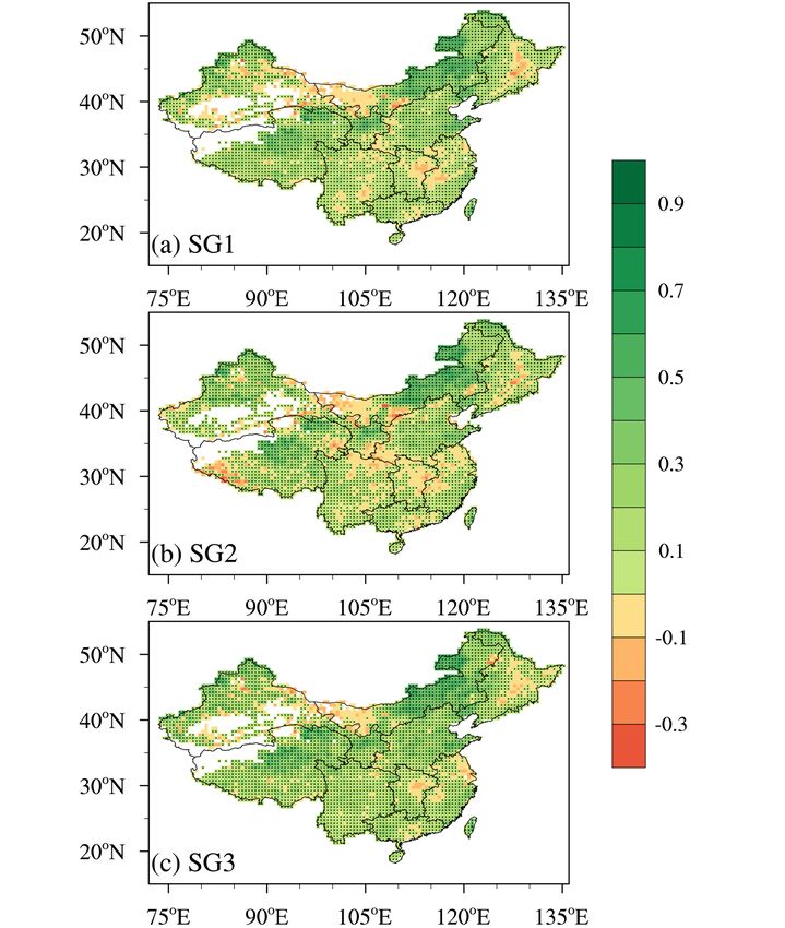
Figures

 Figure S1. Spatial patterns of temporal correlation coefficients between annual GPP from MTE and
 that from ensemble mean of MsTMIP simulations for the period of 1982–2010, including: (a) SG1, (b)
5 SG2, and (c) SG3. Stippling highlights regions with significant correlations (p < 0.05).

 3

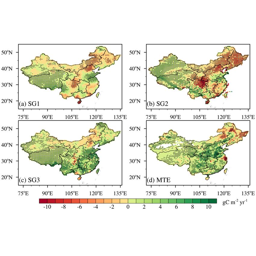
Figure S2. Trends in annual GPP between 1982 and 2010 from the ensemble mean of MsTMIP
 simulations: (a) SG1, (b) SG2, (c) SG3 and (d) MTE. Stippling highlights regions with significant
 trend (p < 0.05).
5

 4

References

 Ahlström, A., Raupach, M., Schurgers, G., Smith, B., Arneth, A., Jung, M., Reichstein, M., Canadell,
 J., Friedlingstein, P., Jain, A., Kato, E., Poulter, B., Sitch, S., Stocker, B., Viovy, N., Wang, Y.,
 Wiltshire, A., Zaehle, S., and Zeng, N.: The dominant role of semi-arid ecosystems in the trend and
 5 variability of the land CO2 sink, Science, 348(6237), 895–899, 2015.
 Baker, I. T., Prihodko, L., Denning, A. S., Goulden, M., Miller, S. and da Rocha, H. R.: Seasonal
 drought stress in the Amazon: reconciling models and observations, J. Geophys. Res., 113, G00B01,
 doi: 10.1029/2007JG000644, 2008.
 Chen, M., Rafique, R., Asrar, G. R., Bond-Lamberty, B., Ciais, P., Zhao, F., Reyer, C. P. O., Ostberg,
10 S., Chang, J., Ito, A., Yang, J., Zeng, N., Kalnay, E., West, T., Leng, G., Francois, L., Munhoven, G.,
 Henrot, A., Tian, H., Pan, S., Nishina, K., Viovy, N., Morfopoulos, C., Betts, R., Schaphoff, S.,
 Steinkamp, J., and Hickler, T.: Regional contribution to variability and trends of global gross primary
 productivity, Environ. Res. Lett., 12, 105005, 2017.
 Hayes, D. J., McGuire, A. D., Kicklighter, D. W., Gurney, K. R., Burnside, T. J. and Melillo, J. M.: Is
15 the northern high-latitude land-based CO2 sink weakening? Global Biogeochem. Cycles, 25, GB3018,
 doi: 10.1029/2010GB003813, 2011.
 Huntzinger, D. N., Schwalm, C., Michalak, A. M., Schaefer, K., King, A. W., Wei, Y., Jacobson, A.,
 Liu, S., Cook, R. B., Post, W. M., Berthier, G., Hayes, D., Huang, M., Ito, A., Lei, H., Lu., C., Mao.,
 J., Peng, C. H., Peng, S., Poulter, B., Ricciuto, D., Shi, X., Tian, H., Wang, W., Zeng, N., Zhao, F.,
20 and Zhu, Q.: The North American Carbon Program Multi-scale Synthesis and Terrestrial Model
 Intercomparison Project: Part 1: overview and experimental design, Geosci. Model Dev. 6, 2121–2133,
 2013.
 Hurtt, G. C., Chini, L., Frolking, S., Betts, R., Edmonds, J., Feddema, J., Fisher, G., Goldewijk, K. K.,
 Hibbard, K., Houghton, R., Janetos, A., Jones, C., Kinderman, G., Konoshita, T., Riahi, K.,
25 Shevliakova, E., Smith, S. J., Stefest, E., Thomson, A. M., Thornton, P., van Vuuren, D., and Wang,
 Y.: Harmonization of land-use scenarios for the period 1500–2100: 600 years of global gridded annual
 land-use transitions, wood harvest, and resulting secondary lands, Clim. Change, 109, 117–161,
 doi:10.1007/s10584-011-0153-2, 2011.
 Ito, A., and Inatomi, M.: Water-use efficiency of the terrestrial biosphere: A model analysis focusing
30 on interactions between the global carbon and water cycles, J. Hydrometeorol., 13(2), 681–694, 2012.
 Jain, A. K., Meiyappan, P., Song, Y., and House, J.: CO2 emissions from land-use change affected
 more by nitrogen cycle, than by the choice of land-cover data, Global Change Biol., 19, 2893–2906,
 doi: 10.1111/gcb.12207, 2013.

 5

Jung, M., Henkel, K., Herold, M., and Churkina, G.: Exploiting synergies of global land cover products
 for carbon cycle modeling, Remote Sens. Environ., 101, 534–553, doi:10.1016/j.rse.2006.01.020,
 2006.
 Krinner, G., Viovy, N., de Noblet-Ducoudré , N., Ogée, J., Polcher, J., Friedlingstein, P., Ciais, P.,
 5 Sitch, S., and Prentice, I. C.: A dynamic global vegetation model for studies of the coupled atmosphere-
 biosphere system, Global Biogeochem. Cycles, 19, GB1015, doi: 10.1029/2003GB002199, 2005.
 Lei, H., Huang, M., Leung, L. R., Yang, D., Shi, X. Mao, J., Hayes, D. H., Schwalm, C. R., Wei, Y.,
 and Liu, S.: Sensitivity of global terrestrial gross primary production to hydrologic states simulated by
 the community land model using two runoff parameterizations, J. Adv. Model Earth Syst., 6, 658–679,
10 2014.
 Mao, J., Thornton, P. E., Shi, X., Zhao, M. and Post, W. M.: Remote sensing evaluation of CLM4 GPP
 for the period 2000–09, J. Clim., 25, 5327–5342, doi:10.1175/JCLI-D-11-00401.1, 2012.
 Piao, S., Fang, J., Ciais, P., Peylin, P., Huang, Y., Sitch, S., and Wang, T.: The carbon balance of
 terrestrial ecosystems in China, Nature, 458, 1009–1013, 2009.
15 Ricciuto, D. M., King, A. W., Dragoni, D. and Post, W. M.: Parameter and prediction uncertainty in
 an optimized terrestrial carbon cycle model: effects of constraining variables and data record length,
 J. Geophys. Res., 116, G01033. doi: 10.1029/2010JG001400, 2011.
 Schaefer, K., Collatz, G. J., Tans, P., Denning, A. S., Baker, I., Berry, J., Prihodko, L., Suits, N., and
 Philpott, A.: Combined Simple Biosphere/Carnegie-Ames-Stanford Approach terrestrial carbon cycle
20 model, J. Geophys. Res., 113, G03034, doi: 10.1029/2007JG000603, 2008.
 Sen, P. K.: Estimates of the regression coefficient based on Kendall’s tau, J. Amer. Stat. Assoc., 63,
 1379–1389, 1968.
 Shi, X., Mao, J., Thornton, P. E., Hoffman, F. M. and Post, W. M.: The impact of climate, CO2,
 nitrogen deposition and land use change on simulated contemporary global river flow, Geophys. Res.
25 Lett., 38, L08704. doi: 10.1029/2011GL046773, 2011.
 Sitch, S., Smith, B., Prentice, I. C., Arneth, A., Bondeau, A., Cramer, W., Kaplans, J. O., Levis, S.,
 Lucht, W., Sykes, M. T., Thonicke, K., and Venevsky, S.: Evaluation of ecosystem dynamics, plant
 geography and terrestrial carbon cycling in the LPJ dynamic global vegetation model, Global Change
 Biol., 9, 161–185, 2003.
30 Tian, H., Chen, G., Zhang, C., Liu, M., Sun, G., Chappelka, A., Ren, W., Xu, X., Lu, C., Pan, S., Chen,
 H., Hui, D., McNulty, S., Lockaby, G., and Vance, E.: Century-scale responses of ecosystem carbon
 storage and flux to multiple environmental changes in the southern United States, Ecosystems, 15,
 674–694, 2012.

 6

Tian, H., Xu, X., Lu, C., Liu, M., Ren, W., Chen, G., Melillo, J., and Liu, J.: Net exchanges of CO2,
 CH4, and N2O between China’s terrestrial ecosystems and the atmosphere and their contributions to
 global climate warming, J. Geophys. Res. 116, G02011, doi: 10.1029/2010JG001393, 2011.
 Wei, Y., Liu, S., Huntzinger, D. N., Michalak, A. M., Viovy, N., Post, W. M., Schwalm, C. R.,
 5 Schaefer, K., Jacobson, A., Lu., C., Tian, H., Ricciuto, D., Cook, R. B., Mao., J., and Shi, X.: The
 North American Carbon Program Multi-scale Synthesis and Terrestrial Model Intercomparison
 Project–Part 2: Environmental driver data, Geosci. Model Dev. 7, 2875–2893, 2014a.
 Wei, Y., Liu, S., Huntzinger, D. N., Michalak, A. M., Viovy, N., Post, W. M., Schwalm, C. R.,
 Schaefer, K., Jacobson, A. R., Lu, C., Tian, H., Ricciuto, D.M., Cook, R.B., Mao, J., and Shi, X.:
10 NACP MsTMIP: Global and North American Driver Data for Multi-Model Intercomparison, ORNL
 DAAC, Oak Ridge, Tennessee, USA. https://doi.org/10.3334/ORNLDAAC/1220, 2014b.
 Zeng, N., Mariotti, A. and Wetzel, P.: Terrestrial mechanisms of interannual CO2 variability, Global
 Biogeochem. Cycles, 19, GB1016, doi: 10.1029/2004GB002273, 2005.

 7