Supplement of Oceanic CO2 outgassing and biological production hotspots induced by pre-industrial river loads of nutrients and carbon in a global ...
←
→
Page content transcription
If your browser does not render page correctly, please read the page content below
Supplement of Biogeosciences, 17, 55–88, 2020
https://doi.org/10.5194/bg-17-55-2020-supplement
© Author(s) 2020. This work is distributed under
the Creative Commons Attribution 4.0 License.

Supplement of
Oceanic CO2 outgassing and biological production hotspots induced by
pre-industrial river loads of nutrients and carbon in a global modeling
approach
Fabrice Lacroix et al.

Correspondence to: Fabrice Lacroix (fabrice.lacroix@mpimet.mpg.de)

The copyright of individual parts of the supplement might differ from the CC BY 4.0 License.
S.1 Methods: Inputs to catchments
S.1.1 Anthropogenic P inputs
In this study, we assumed anthropogenic inputs from agricultural, sewage and allochtonous P sources. The anthropogenic
sources were distributed according to anthropogenic exports of present-day NEWS2 DIP exports. To verify that this assumption
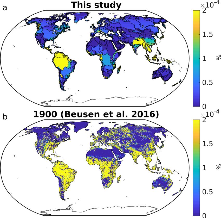
5 is plausible, we compared our assumed distribution (Figure 1a) to the distributions of anthropogenic P inputs to catchments of
the modelling study of Beusen et al. (2016), which account for 1900 (Figure 1b) to the year 2000 (Figure 1c). The results show
that the present-day anthropogenic DIP distributions assumed in our study strongly agree with both the Beusen et al. (2016) for
year 1900 and 2000. We furthermore observe very similar distributions of anthropogenic inputs to catchments for year 1900
and 2000 in the Beusen et al. (2016) study, although increasing contributions to P inputs in Southeast Asia can be observed.
10 Nevertheless, we acknowledge that pre-industrial anthropogenic exports are likely strongly uncertain in their magnitudes as
well as in their distributions due to the lack of data.
1
Figure 1. Relative contributions of anthropogenic P inputs to catchments [10-4 %] as assumed in our study (a), as well as for year 1900 (b)
and 2000 as assumed in Beusen et al. (2016). This was calculated for every grid cell of a regular 720x360 grid.

                                                                    2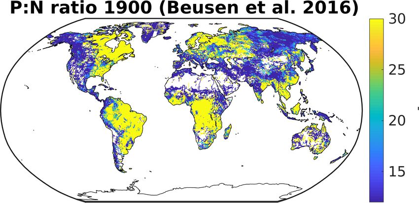
S.1.2 Allochthonous P inputs

     The distributions of allochthonous P riverine exports was assumed to be the same as organic matter riverine exports, which were
     derived from the NEWS2 study. This was done primarily in order to avoid having strongly differing organic matter exports to
     total P exports, which would be problematic in our fractionation assumptions for P. For instance, if organic matter exports were
5    very high and P inputs were very low, all P would be assumed to be transformed to organic matter, leaving DIP exports close
     to null. Comparing our assumed distribution with the distribution from Beusen et al. (2016) however reveals a strong level of
     agreement, signaling that the allochtonous inputs to catchments might be strongly correlated to net organic matter production
     within the catchments.

     Figure 2. Relative contributions of allochthonous inputs to catchments as assumed in our study (a) and of 1900 inputs assumed in Beusen
     et al. (2016). This was calculated for every grid cell of a regular 720x360 grid.

     S.1.3 N:P ratios

10   In this study, we assume riverine N:P mole ratios of 16:1 for dissolved inorganic as well as organic species. In literature, higher
     values for this ratio can be found. For one, Beusen et al. (2016) simulate a mole N:P ratio for total exports to the ocean of around
     21:1 both for 1900 as well as for present-day. Meybeck (1982) suggest a DIN:DIP mole ratio of 26:1 based on observational
     data from major rivers (contemporary) and Seitzinger et al. (2010) model a DIN:DIP ratio of present-day ratio of 29:1. DIN has
     however been reported to have undergone stronger increases than DIP, atleast since 1970 (Seitzinger et al., 2010). Seitzinger
15   et al. (2010) simulate a global DON:DOP mole ratio of 39:1. Meybeck (1982) also suggest a total organic N:P export mole
     ratio of around 9:1, albeit with acknowledgly relatively little observational data.

                                                                       3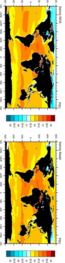
While higher N:P values are reported in literature, denitrification in estuaries and in the coastal ocean likely compensate for
    the higher N:P ratio by elimating DIN, with estimations of the denitrification flux being around 3-10 Tg N yr-1 .
       The total additional riverine N export (7 Tg N yr-1 ) when using for instance a ratio of 21:1 (Beusen et al., 2016) could there-
    fore be completly offset by the loss of nitrogen in estuaries. When accounting for denitrification in estuaries, the difference in
5   the global N export would be small (-14-10 %). Regionally however, differing N:P ratios could have strong impacts, especially
    when considering the anthropogenic of riverine exports. For instance, Beusen et al. (2016) show much higher N:P ratios on the
    South American continent, eastern North America, Northern Europe and Southeast Asia.

    Figure 3. N:P ratio catchment inputs modelled in Beusen et al. (2016).

                                                                        4
S.2 Methods: HAMOCC Model parameters
S.2.1 Comparison with standard parameters
Table 1. Comparison of main model parameters with Ilyina et al. (2013). Model equations can be found in Ilyina et al. (2013), as well as
Paulsen et al. (2017) for the implementation of cyanobacteria in the model.
Symbol Variable This study Ilyina et al., 2013 Units
Phytoplankton
αphy Initial slope of the photosynthesis versus the irradiance curve 0.03 0.03 m2 W-1 d-1
µphy Maximum growth rate 0.6 0.6 d-1
Phymin Minimum Concentration of phytoplankton 1E-11 1E-11 kmol P m-3
λphy Mortality rate 0.008 0.008 d-1
β phy Exudation rate 0.03 0.03 d-1
Cyanobacteria
αcya Initial slope of the photosynthesis versus the irradiance curve 0.02 - m2 W-1 d-1
µcya Maximum growth rate 0.2 - d-1
◦
Topt Optimal growth temperature 28 - C
◦
T1 , T2 Temperature distribution parameters 5.5, 1 - C
Cyamin Minimum Concentration of cyanobacteria 1E-11 - kmol P m-3
λphy Mortality rate 0.1 - d-1
β cya Exudation rate 0.01 - d-1
Zooplankton
µZoo Max. Grazing Rate 1 1 d-1
KZoo Half-saturation constant for grazing 4E-8 4E-8 kmol P m-3
Zoomin Min. concentration of zooplankton 1E-11 1E-11 kmol P m-3
1-Zoo Fraction of grazing egested 0.2 0.2 -
λZoo Mortality rate 3E6 3E6 d-1
β Zoo Excretion rate 0.06 0.06 d-1
1-can Fraction of carnivores grazing egested 0.05 0.05 -
Nutrients
KPO4 Half-saturation constant for DIP uptake 4E-8 4E-8 kmol P m-3
KNO3 Half-saturation constant for DIN uptake 1.6E-7 1.6E-7 kmol N m-3
KDFe Half-saturation constant for DFe uptake 0.0036 1.6E-7 kmol N m-3
Rdust Ratio of bioavailable iron in dust 6.26E-6 6.26E-6 kmol Fe kg-1
Fecrit Critical Fe concentration of complexation 5E-10 6E-10 kmol m-3
5Symbol Variable This study Ilyina et al., 2013 Units
Particulate organic matter (POM)
wdet Sinking speed of POM 5 5 d-1
O2crit Aerob threshold 5E-8 5E-8 kmol O2 m-3
λdet Remineralization rate 0.026 0.025 d-1
λN Denitrification rate to N2 O 0.01 0.01 d-1
Rdenit Ratio of DIN consumed in denitrification 137.6 137.6 mol N (mol P)-1
λN Denitrification rate to N 0.005 0.005 d-1
Rdenit Ratio of N2 O consumed in denitrification to N 344 344 mol N (mol P2 )-1
Rnit DIN produced during nitrification 1E-4 1E-4 mol N mol O2 -1
Dissolved organic matter (DOM)
λDOM (Bacterial) remineralization rate 0.008 0.004 d-1
Shell material
KSi Half saturation constant for Si(OH)4 uptake 1E-6 1E-6 kmol Si m-3
RSi:P DSi:P uptake ratio during opal production 25 25 mol Si (mol P)-1
RCa:P DIC:P uptake ratio during CaCO3 production 35 20 mol C (mol P)-1
wopal Sinking speed of opal 30 30 d-1
wcalc Sinking speed of CaCO3 30 30 d-1
λopal Opal dissolution rate 0.01 0.01 d-1
λcalc CaCO3 dissolution rate 0.075 0.075 d-1
6S.2.2 tDOM degradation validation
At a tDOM degradation rate of 0.003 d-1 , 0.39 Tg C yr-1 of riverine tDOM is remineralized on the Lousiana Shelf, whereas
5 0.68 is suggested to be degraded on the shelf in Fichot and Benner (2014). 2.09 Tg C yr-1 is simulated to be degraded in the
Baltic Sea whereas 1.75 Tg C yr-1 is budgeted in Seidel et al. (2017).
The surface tDOM concentrations in the Pacific contribute to less than 1 % of total DOM concentrations in the entire basin,
which is consistent with Lignin measurements in the surface ocean of the North Pacific that suggest tDOM contributions of
around 1% to total DOM Hernes and Benner (2002). In the North Atlantic, the contribution of tDOM to the total DOM is
10 suggested to be higher (around 2.4 %, Opsahl and Benner (1997)), which is also reflected in the model with contributions even
exceeding 5% in some areas of the open ocean.
7S.3 Analysis: Freshwater inputs to the ocean
The freshwater loads from OMIP were already implemented in previous standard HAMOCC version, in order to close the
hydrological cycle. Globally, they add 32,542 km3 yr-1 of freshwater to the ocean. These impact the salinity and the ocean
stratification in the proximity of our biogeochemical riverine inputs, and therefore their advection within the ocean.
Figure 4. Comparison of salinity from observational data (WOA) and modelled salinity in RIV (Salinity Model).
.
8S.4 Analysis: Coastal Profiles
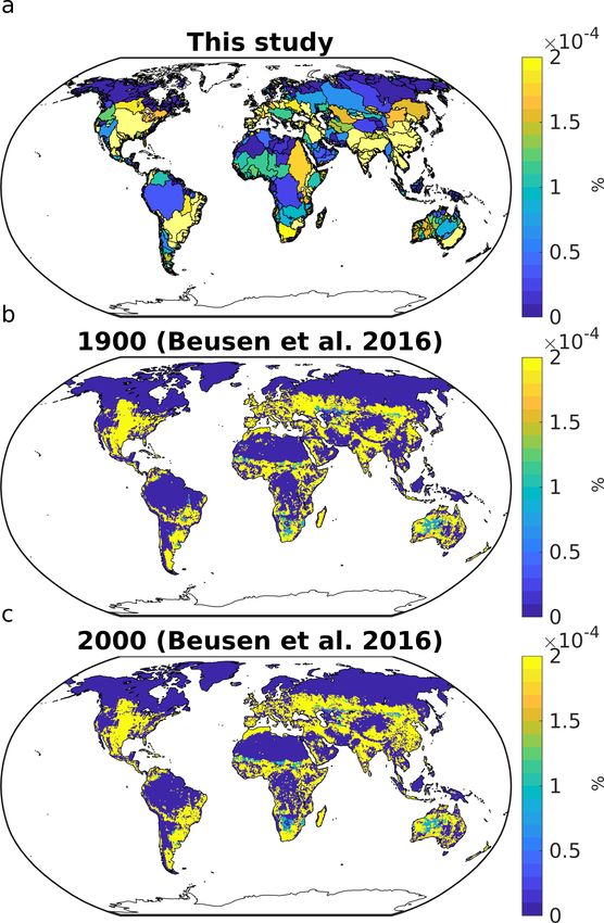
Coastal vertical profiles show that despite the coarse resolution of our model, the features of salinity in selected coastal regions
is comparable to WOA data, although vertical gradients are often not as strong as in the observational data (Figure A.2).
For the Amazon Northward section, we see a vertical the salinity gradient in the WOA data, which is also reproduced albeit
5 not extensively in the modelled data which induces stronger stratification of the water layers. In terms of absolute values the
salinity is also well represented for the Ganges river, although the vertical stratification is also not quite as extensive further
away from the coast. The bathymetry of the Laptev Sea at the Lena river mouth is poorly represented, as WOA data shows
a height increase of the ocean floor at connection of the Sea with the Arctic Ocean, which is not represented in the model
bathymetry. The salinity gradient in the East Chinese Sea is very strong due to currents parallel in the model which are also
10 shown in observations (Ichikawa and Beardsley, 2002). Smaller currents in this region and in the Yellow Sea are however not
well represented in the model. The Congo river has a very steep coastal shelf, and therefore the salinity relatively strong vertical
horizontal gradient, due to little bathymetry induced vertical mixing, as well as heating of the surface waters.
9a f
b g
c h
d i
e j
Figure 5. Vertical profiles of the coastal bathymetry and salinity, along specific longitudes and longitudes for chosen river mouths. The left
column (a-e) is made of WOA salinity profiles, whereas the right column (f-j) of profiles from model simulation RIV. a & f are shelf and
salinity profiles at the Amazon river (TWA), b & g for the Ganges river, c & h Lena river, d & i Yangtze river, e & j Congo river.
10S.5 Analysis: Magnitudes of inputs to the open and coastal ocean in REF
In order to assess the impacts of open ocean biogeochemical inputs (as in the standard model simulation REF) on the dissolved
inorganic nutrient concentrations, we calculated the P inputs to the surface layers and compared them to the surface ocean
(first 12 meters) inventories of 3 regions of the open ocean in the model, as well as for the global coastal ocean (depths of
5 less than 250m). In the productive regions of the equatorial Pacific and in the Southern Ocean, the P inputs are very small in
comparison to the surface P inventories (Figure 2). This signals that the inputs are not strong contributors to maintaining the
DIP concentrations here. In the tropical Atlantic, the inputs might cause a bias by artificially increasing the concentrations. We
however only calculate the inventories in the first 12m inventories here, although primary can take place until up to around
100m in the model. Therefore, the inputs are still likely very small compared to the nutrient inventories that impact the NPP.
10 Throughout our study, we also show that the ocean physics is a much stronger contributor to open ocean biogeochemical
distributions than the locations of the biogeochemical inputs. For instance, the difference between RIV and REF in the open
ocean NPP is relatively small, with the major features being conserved. Considering riverine inputs however impacts certain
coastal regions substantially and could affect certain regions of the open ocean (tropical Atlantic).
The inputs to the coastal ocean are very small in REF (6%), meaning that the vast majority of inputs in the simulation
15 REF happens in the open ocean. In the simulation RIV however, 100% of the inputs are added to the coastal ocean at the
river mouths. Therefore, our simulations allow a comparison between an ocean state where inputs are added to the open ocean
(REF), and one where inputs are added at their correct locations in the coastal ocean.
Table 2. Surface P inputs in REF in relation to surface DIP concentrations (first 12 m).
Region P inputs (percentage of global input) Surface layer DIP inventories Input to inventory ratio
[Tg P yr-1 ] Tg P
Open equatorial Pacific 0.33 (9%) 5.15 6%
Open equatorial Atlantic 0.12 (3%) 0.41 29%
Southern Ocean 0.20 (6%) 9.82 2%
Coastal Ocean 0.19 (6%) 3.08 6%
11References
Beusen, A. H. W., Bouwman, A. F., Van Beek, L. P. H., Mogollón, J. M., and Middelburg, J. J.: Global riverine N and P transport
to ocean increased during the 20th century despite increased retention along the aquatic continuum, Biogeosciences, 13, 2441–2451,
https://doi.org/10.5194/bg-13-2441-2016, 2016.
5 Fichot, C. G. and Benner, R.: The fate of terrigenous dissolved organic carbon in a river-influenced ocean margin, Global Biogeochemical
Cycles, 28, 300–318, https://doi.org/10.1002/2013GB004670, 2014.
Hernes, P. J. and Benner, R.: Transport and diagenesis of dissolved and particulate terrigenous organic matter in the North Pacific Ocean,
Deep Sea Research Part I: Oceanographic Research Papers, 49, 2119–2132, https://doi.org/https://doi.org/10.1016/S0967-0637(02)00128-
0, http://www.sciencedirect.com/science/article/pii/S0967063702001280, 2002.
10 Ichikawa, H. and Beardsley, R. C.: The Current System in the Yellow and East China Seas, Journal of Oceanography, 58, 77–92,
https://doi.org/10.1023/A:1015876701363, 2002.
Ilyina, T., Six, K. D., Segschneider, J., Maier-Reimer, E., Li, H., and NúñezRiboni, I.: Global ocean biogeochemistry model HAMOCC:
Model architecture and performance as component of the MPI-Earth system model in different CMIP5 experimental realizations, Journal
of Advances in Modeling Earth Systems, 5, 287–315, https://doi.org/10.1029/2012MS000178, 2013.
15 Meybeck, M.: Carbon, Nitrogen, and Phosphorus Transport by World Rivers, Am. J. Sci., 282, 1982.
Opsahl, S. and Benner, R.: Distribution and cycling of terrigenous dissolved organic matter in the ocean, Nature, 386, 480–482,
https://doi.org/10.1038/386480a0, https://doi.org/10.1038/386480a0, 1997.
Paulsen, H., Ilyina, T., Six, K. D., and Stemmler, I.: Incorporating a prognostic representation of marine nitrogen fixers into the global ocean
biogeochemical model HAMOCC, Journal of Advances in Modeling Earth Systems, 9, 438–464, https://doi.org/10.1002/2016MS000737,
20 2017.
Seidel, M., Manecki, M., Herlemann, D. P. R., Deutsch, B., Schulz-Bull, D., Jürgens, K., and Dittmar, T.: Composition and Transformation
of Dissolved Organic Matter in the Baltic Sea, Frontiers in Earth Science, 5, 1–20, https://doi.org/10.3389/feart.2017.00031, 2017.
Seitzinger, S. P., Mayorga, E., Bouwman, A. F., Kroeze, C., Beusen, A. H. W., Billen, G., Drecht, G. V., Dumont, E., Fekete, B. M., Garnier,
J., and Harrison, J. A.: Global river nutrient export: A scenario analysis of past and future trends, Global Biogeochemical Cycles, 24,
25 https://doi.org/10.1029/2009GB003587, 2010.
12You can also read