Localizing Visual Sounds the Hard Way
←
→
Page content transcription
If your browser does not render page correctly, please read the page content below
Localizing Visual Sounds the Hard Way

                                                               Honglie Chen, Weidi Xie, Triantafyllos Afouras, Arsha Nagrani
                                                                           Andrea Vedaldi, Andrew Zisserman
                                                             {hchen, weidi, afourast, arsha, vedaldi, az}@robots.ox.ac.uk
                                                            VGG, Department of Engineering Science, University of Oxford, UK
                                                            http://www.robots.ox.ac.uk/˜vgg/research/lvs/
arXiv:2104.02691v1 [cs.CV] 6 Apr 2021

                                        Figure 1: Visual Sound Source Localisation: We localise sound sources in videos without manual annotation. Our key
                                        contribution is an automatic negative mining technique through differentiable thresholding of a cross-modal correspondence
                                        score map, the background regions with low correlation to the given sound as ‘hard negatives’, and the regions in the Tri-map
                                        is‘ignored’ in a contrastive learning framework.

                                                                Abstract                                 1. Introduction

                                           The objective of this work is to localize sound sources          While research in computer vision largely focuses on the
                                        that are visible in a video without using manual annota-         visual aspects of perception, natural objects are character-
                                        tions. Our key technical contribution is to show that, by        ized by much more than just appearance. Most objects,
                                        training the network to explicitly discriminate challenging      in particular, emit sounds, either in their own right, or in
                                        image fragments, even for images that do contain the ob-         their interaction with the environment — think of the bark
                                        ject emitting the sound, we can significantly boost the lo-      of a dog, or the characteristic sound of a hammer striking
                                        calization performance. We do so elegantly by introducing        a nail. A full understanding of natural objects should not
                                        a mechanism to mine hard samples and add them to a con-          ignore their acoustic characteristics. Instead, modelling ap-
                                        trastive learning formulation automatically. We show that        pearance and acoustics jointly can often help us understand
                                        our algorithm achieves state-of-the-art performance on the       them better and more efficiently. For example, several au-
                                        popular Flickr SoundNet dataset. Furthermore, we intro-          thors have shown that it is possible to use sound to discover
                                        duce the VGG-Sound Source (VGG-SS) benchmark, a new              and localize objects automatically in videos, without the use
                                        set of annotations for the recently-introduced VGG-Sound         of any manual supervision [1, 2, 15, 18, 25, 31].
                                        dataset, where the sound sources visible in each video clip         In this paper, we consider the problem of localizing ‘vi-
                                        are explicitly marked with bounding box annotations. This        sual sounds’, i.e. visual objects that emit characteristics
                                        dataset is 20 times larger than analogous existing ones,         sounds in videos. Inspired by prior works [2, 15, 31], we
                                        contains 5K videos spanning over 200 categories, and, dif-       formulate this as finding the correlation between the visual
                                        ferently from Flickr SoundNet, is video-based. On VGG-SS,        and audio streams in videos. These papers have shown that
                                        we also show that our algorithm achieves state-of-the-art        not only can this correlation be learned successfully, but
                                        performance against several baselines.                           that, once this is done, the resulting convolutional neural
                                                                                                         networks can be ‘dissected’ to localize the sound source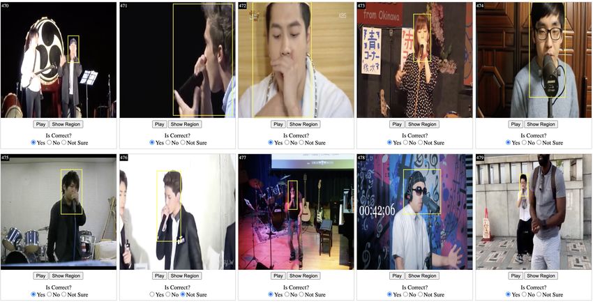
spatially, thus imputing it to a specific object. However,           2. Related Work
other than in the design of the architecture itself, there is lit-
tle in this prior work meant to improve the localization capa-       2.1. Audio-Visual Sound Source Localization
bilities of the resulting models. In particular, while several           Learning to localize sound sources by exploiting the nat-
models [1, 2, 31] do incorporate a form of spatial attention         ural co-occurrence of visual and audio cues in videos has
which should also help to localize the sounding object as a          a long history. Early attempts to solve the task used shal-
byproduct, these may still fail to provide a good coverage           low probabilistic models [9, 17, 21], or proposed segment-
of the object, often detecting too little or too much of it.         ing videos into spatio-temporal tubes and associating those
    In order to address this issue, we propose a new training        to the audio signal through canonical correlation analysis
scheme that explicitly seeks to spatially localize sounds in         (CCA) [19].
video frames. Similar to object detection [36], in most cases            Modern approaches solve the problem using deep neu-
only a small region in the image contains an object of inter-        ral networks — typically employing a dual stream, trained
est, in our case a ‘sounding’ object, with the majority of the       with a contrastive loss by exploiting the audio-visual cor-
image often being ‘background’ which is not linked to the            respondence, i.e. matching audio and visual representations
sound. Learning accurate object detectors involves explic-           extracted from the same video. For example, [2, 15, 28, 31]
itly seeking for these background regions, prioritizing those        associate the appearance of objects with their characteris-
that could be easily confused for the object of interest, also       tic sounds or audio narrations; Hu et al. [18] first cluster
called hard negatives [7, 13, 22, 29, 32, 36]. Given that we         audio and visual representations within each modality, fol-
lack supervision for the location of the object making the           lowed by associating the resulting centroids with contrastive
sound, however, we are unable to tell which boxes are pos-           learning; Qian et al. [27] proposed a weakly supervised ap-
itive or negative. Furthermore, since we seek to solve the           proach, where the approximate locations of the objects are
localization rather than the detection problem, we do not            obtained from CAMs to bootstrap the model training. Apart
even have bounding boxes to work with, as we seek instead            from using correspondence, Owens and Efros [26] also lo-
a segmentation of the relevant image area.                           calize sound sources through synchronization, a related ob-
                                                                     jective also investigated in earlier works [6, 23], while [20]
   In order to incorporate hard evidence in our unsupervised         incorporate explicit attention in this model. Afouras et
(or self-supervised) setting, we propose an automatic back-          al. [1] also exploit audio-visual concurrency to train a video
ground mining technique through differentiable threshold-            model that can distinguish and group instances of the same
ing, i.e. regions with low correlation to the given sound are        category.
incorporated into a negatives set for contrastive learning. In-          Alternative approaches solve the task using an audio-
stead of using hard boundaries, we note that some regions            visual source separation objective. For example Zhao et
may be uncertain, and hence we introduce the concept of              al. [39] employ a mix-and-separate approach to learn to as-
a Tri-map into the training procedure, leaving an ‘ignore’           sociate pixels in video frames with separated audio sources,
zone for our model. To our knowledge, this is the first              while Zhao et al. [38] extends this method by providing the
time that background regions have been explicitly consid-            model with motion information through optical flow. Rou-
ered when solving the sound source localization problem.             ditchenko et al. [30] train a two-stream model to co-segment
We show that this simple change significantly boosts sound           video and audio, producing heatmaps that roughly highlight
localization performance on standard benchmarks, such as             the object according to the audio semantics. These methods
Flickr SoundNet [31].                                                rely on the availability of videos containing single-sound
    To further assess sound localization algorithms, we              sources, usually found in well curated datasets. In other re-
also introduce a new benchmark, based on the recently-               lated work, Gan et al. [10] learn to detect cars from stereo
introduced VGG-Sound dataset [4], where we provide high-             sound, by distilling video object detectors, while Gao et
quality bounding box annotations for ‘sounding’ objects,             al. [11] lift mono sound to stereo by leveraging spatial in-
i.e. objects that produce a sound, for more than 5K videos           formation.
spanning 200 different categories. This dataset is 20×
                                                                     2.2. Audio-Visual Localization Benchmarks
larger and more diverse than existing sound localization
benchmarks, such as Flickr SoundNet (the latter is also                 Existing audio-visual localization benchmarks are sum-
based on still images rather than videos). We believe this           marised in Table 1 (focusing on the test sets). The Flickr
new benchmark, which we call VGG-Sound Source, or                    SoundNet sound source localization benchmark [31] is an
VGG-SS for short, will be useful for further research in this        annotated collection of single frames randomly sampled
area. In the experiments, we establish several baselines on          from videos of the Flickr SoundNet dataset [3, 34]. It
this dataset, and further demonstrate the benefits of our new        is currently the standard benchmark for the sound source
algorithm.                                                           localization task; we discuss its limitations in Section 4,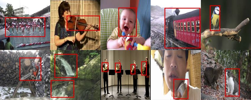
where we introduce our new benchmark. The Audio-Visual             certain regions effectively.
Event (AVE) dataset [35], contains 4,143 10 second video               In sections 3.1 to 3.3 we first describe the task of audio-
clips spanning 28 audio-visual event categories with tem-          visual localization using contrastive learning in its oracle
poral boundary annotations. LLP [37] contains of 11,849            setting, assuming, for each visual-audio pair, we do have
YouTube video clips spanning 25 categories for a total of          the ground-truth annotation for which region in the image
32.9 hours collected from AudioSet [12]. The development           is emitting the sound. In section 3.4, we introduce our pro-
set is sparsely annotated with object labels, while the test set   posed idea, which replaces the oracle, and discuss the dif-
contains dense video and audio sound event labels on the           ference between our method and existing approaches.
frame level. Note that the AVE and LLP test sets contain
only temporal localisation of sounds (at the frame level),         3.1. Audio-Visual Feature Representation
with no spatial bounding box annotation.                              Given a short video clip with N visual frames and audio,
                                                                   and considering the center frame as visual input, i.e. X =
 Benchmark Datasets      # Data    # Classes   Video    BBox       {I, a}, I ∈ R3×Hv ×Wv , a ∈ R1×Ha ×Wa . Here, I refers
                                                                   to the visual frame, and a to the spectrogram of the raw
 Flickr SoundNet [31]      250       ∼50‡        ×        X
                                                                   audio waveform. In this manner, representations for both
 AVE [35]†                 402        28         X        ×
                                                                   modalities can be computed by means of CNNs, which we
 LLP [37]†                1,200       25         X        ×
 VGG-SS                   5,158      220         X        X        denote respectively f (·; θ1 ) and g(·; θ2 ). For each video Xi ,
                                                                   we obtain visual and audio representations:
Table 1: Comparison with the existing sound-source locali-                       Vi = f (Ii ; θ1 ),   Vi ∈ Rc×h×w ,             (1)
sation benchmrks. Note that VGG-SS has more images and                                                        c
classes. †These datasets contain only temporal localisation                      Ai = g(ai ; θ2 ),    Ai ∈ R .                  (2)
of sounds, not spatial localisation. ‡ We determined this via      Note that both visual and audio representation have the
manual inspection.                                                 same number of channels c, which allows to compare them
                                                                   by using dot product or cosine similarity. However, the
3. Method                                                          video representation also has a spatial extent h × w, which
                                                                   is essential for spatial localization.
    Our goal is to localize objects that make characteristic
sounds in videos, without using any manual annotation.             3.2. Audio-Visual Correspondence
Similar to prior work [2], we use a two-stream network                Given the video and audio representations of eqs. (1)
to extract visual and audio representations from unlabelled        and (2), we put in correspondence the audio of clip i with
video. For localization, we compute the cosine similarity          the image of clip j by computing the cosine similarity of the
between the audio representation and the visual represen-          representations, using the audio as a probe vector:
tations extracted convolutionally at different spatial loca-
tions in the images. In this manner, we obtain a positive                               hAi , [Vj ]:uv i
signal that pulls together sounds and relevant spatial loca-             [Si→j ]uv =                     ,   uv ∈ [h] × [w].
                                                                                       kAi k k[Vi ]:uv k
tions. For learning, we also need an opposite negative sig-
nal. A weak one is obtained by correlating the sound to            This results in a map Si→j ∈ Rh×w indicating how strongly
locations in other, likely irrelevant videos. Compared to          each image location in clip j responds to the audio in clip i.
prior work [1, 2], our key contribution is to also explicitly      To compute the cosine similarity, the visual and audio fea-
seek for hard negative locations that contain background or        tures are L2 normalized. Note that we are often interested
non-sounding objects in the same images that contain the           in correlating images and audio from the same clip, which
sounding ones, leading to more selective and thus precise          is captured by setting j = i.
localization. An overview of our architecture can be found
                                                                   3.3. Audio-Visual Localization with an Oracle
in Figure 2.
    While the idea of using hard negatives is intuitive, an ef-       In the literature, training models for audio-visual lo-
fective implementation is less trivial. In fact, while we seek     calization has been treated as learning the correspondence
for hard negatives, there is no hard evidence for whether          between these two signals, and formulated as contrastive
any region is in fact positive (sounding) or negative (non-        learning [1, 2, 18, 27, 31].
sounding) as videos are unlabelled. An incorrect classi-              Here, before diving into the self-supervised approach,
fication of a region as positive or negative can throw off         we first consider the oracle setting for the contrastive
the localization algorithm entirely. We solve this problem         learning where ground-truth annotations are available.
by using a robust contrastive framework that combines soft         This means that we are given a training set D =
thresholding and Tri-maps, which enables us to handle un-          {d1 , d2 , . . . , dk }, where each training sample di =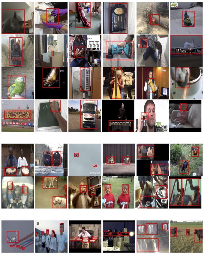
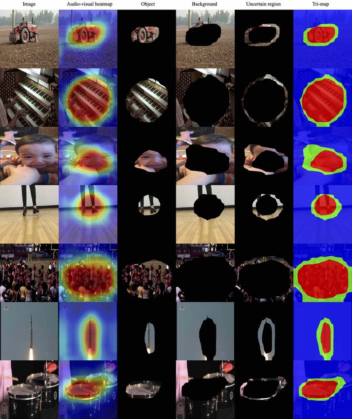
Figure 2: Architecture Overview. We use an audio-visual pair as input to a dual-stream network shown in (a), f (·; θ1 ) and
g(·; θ2 ), denoting the visual and audio feature extractor respectively. Cosine similarity between the audio vector and visual
feature map is then computed, giving us a heatmap of size 14 × 14. (b) demonstrates the soft threshold being applied twice
with different parameters, generating positive, negative regions. The final Tri-map and the uncertain region are highlighed in
(c).
(Xi , mi ) consists of a audio-visual sample Xi , as given          and negative sets. For example, in [31] a heatmap generated
above, plus a segmentation mask mi ∈ Bh×w with ones for             by using the soft-max operator is used to pool the positives
those spatial locations that overlap with the object that emits     and images from other video clips are treated as negatives;
the sounds, and zeros elsewhere. During training, the goal is       instead, in [2], positives come from max pooling the corre-
therefore to jointly optimize f (·; θ1 ) and g(·; θ2 ), such that   spondence map, Si→i and the negatives from max pooling
Si→i gives high responses only for the region that emits the        Si→j for j 6= i. Crucially, all such approaches have missed
sound present in the audio. In this paper, we consider a spe-       the hard negatives term defined above, computed from the
cific type of contrastive learning, namely InfoNCE [14, 24].        background regions within the same images that do con-
                                                                    tain the sound. Intuitively this term is important to obtain
Optimization. For each clip i in the dataset (or batch), we
                                                                    a shaper visual localization of the sound source; however,
define the positive and negative responses as:
                                                                    while this is easy to implement in the oracle setting, obtain-
         1                                                          ing hard negatives in self-supervised training requires some
   Pi =      hmi , Si→i i,                                          care, as discussed next.
       |mi |
           1                           1 X                          3.4. Self-supervised Audio-Visual Localization
  Ni =            h1 − mi , Si→i i +          h1, Si→j i .
       |1 − mi |                     hw
       |            {z          }        i6=j                          In this section, we describe a simple approach for replac-
               hard negatives
                                     |        {z      }
                                             easy negatives         ing the oracle, and continuously bootstrapping the model to
                                                                    achieve better localization results. At a high level, the pro-
where h·, ·i denotes Frobenius inner product. To interpret          posed idea inherits the spirit of self-training, where predic-
this equation, note that the inner product simply sums over         tions are treated as pseudo-ground-truth for re-training.
the element-wise product of the specified tensors and that 1           Specifically, given a dataset D = {X1 , X2 , . . . , Xk }
denotes a h × w tensor of all ones. The first term in the ex-       where only audio-visual pairs are available (but not the
pression for Ni refers to the hard negatives, calculated from       masks mi ), the correspondence map Si→i between audio
the “background” (regions that do not emit the characteris-         and visual input can be computed in the same manner as
tic sound) within the same image, and the second term de-           section 3.2. To get the pseudo-ground-truth mask m̂i , we
notes the easy negatives, coming from other images in the           could simply threshold the map Si→i :
dataset. The optimization objective can therefore be defined                                 (
as:                                                                                            1, if Si→i ≥
                                                                                       m̂i =
                                                                                               0, otherwise
                 k
              1X             exp(Pi )
          L=−       log                                             Clearly, however, this thresholding, which uses the Heav-
              k i=1     exp(Pi ) + exp(Ni )
                                                                    iside function, is not differentiable. Next, we address this
Discussion. Several existing approaches [1, 2, 15, 31] to           issue by relaxing the thresholding operator.
self-supervised audio-visual localization are similar. The          Smoothing the Heaviside function. Here, we adopt a
key difference lies in the way of constructing the positive         smoothed thresholding operator in order to maintain the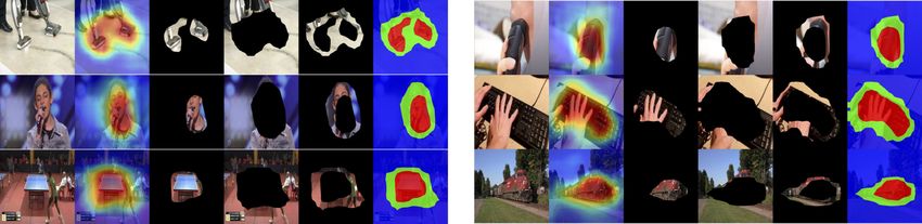
end-to-end differentiability of the architecture:                 4.1. Test Set Annotation Pipeline
                m̂i = sigmoid((Si→i − )/τ )                         In the following sections, we describe a semi-automatic
                                                                  procedure to annotate the objects that emit sounds with
where  refers to the thresholding parameter, and τ denotes       bounding boxes, which we apply to obtain VGG-SS with
the temperature controlling the sharpness.                        over 5k video clips, spanning 220 classes.
Handling uncertain regions. Unlike the oracle setting,            (1) Automatic bbox generation. We use the entire VGG-
the pseudo-ground-truth obtained from the model predic-           Sound test set, containing 15k 10-second video clips, and
tion may potentially be noisy, we therefore propose to set up     extract the center frame from each clip. We use a Faster
an “ignore” zone between the positive and negative regions,       R-CNN object detector [29] pretrained on OpenImages to
allowing the model to self-tune. In the image segmentation        predict the bounding boxes of all relevant objects. Follow-
literature, this is often called a Tri-map and is also used for   ing [4], we use a word2vec model to match visual and audio
matting [5, 33]. Conveniently, this can be implemented by         categories that are semantically similar. At this stage, there
applying two different ’s, one controlling the threshold for     are roughly 8k frames annotated automatically.
the positive part and the other for the negative part of the
Tri-map.                                                          (2) Manual image annotation. We then annotate the re-
                                                                  maining frames manually. There are three main challenges
Training objective. We are now able to replace the oracle         at this point: (i) there are cases where localization is ex-
while computing the positives and negatives automatically.        tremely difficult or impossible, either because the object is
This leads to our final formulation:                              not visible (e.g. in extreme lighting conditions), too small
                                                                  (‘mosquito buzzing’), or is diffused throughout the frame
 m̂ip = sigmoid((Si→i − p )/τ )
                                                                  (‘hail’, ‘sea waves’, ‘wind’); (ii) the sound may originate ei-
 m̂in = sigmoid((Si→i − n )/τ )                                  ther from a single object, or from the interactions between
           1                                                      multiple objects and a consistent annotation scheme must
   Pi =         hm̂ip , Si→i i
        |m̂ip |                                                   be decided upon; and finally (iii), there could be multiple
             1                             1 X                    instances of the same class in the same frame, and it is
  Ni =               h1 − m̂in , Si→i i +      h1, Si→j i         challenging to know which of the instances are making the
        |1 − m̂in |                       hw
                                                     j6=i
                                                                  sound from a single image.
               k
           1   X                exp(Pi )                             We address these issues in three ways: First, we remove
   L=−               log                                          categories (e.g. mainly environmental sounds such as wind,
           k   i=1
                           exp(Pi ) + exp(Ni )
                                                                  hail etc) that are challenging to localize, roughly 50 classes;
where p and n are two thresholding parameters (validated        Second, as illustrated in Figure 3a, when the sound comes
in experiment section), with p > n . For example if we          from the interaction of multiple objects, we annotate a tight
set p = 0.6 and n = 0.4, regions with correspondence            region surrounding the interaction point; Third, if there are
scores above 0.6 are considered positive and bellow 0.4 neg-      multiple instances of the same sounding object category in
ative, while the areas falling within the [0.4, 0.6] range are    the frame, we annotate each separately when there are less
treated as “uncertain” regions and ignored during training        than 5 instances and they are separable, otherwise a single
(Figure 2).                                                       bounding box is drawn over the entire region, as shown in
                                                                  the top left image (‘human crowd’) in Figure 3a.
4. The VGG-Sound Source Benchmark                                 (3) Manual video verification. Finally, we conduct man-
   As mentioned in Section 2, the SoundNet-Flickr sound           ual verification on videos using the VIA software [8]. We
source localization benchmark [31] is commonly used for           do this by watching the 5-second video around every an-
evaluation in this task. However, we found it to be unsat-        notated frame, to ensure that the sound corresponds with
isfactory in the following aspects: i) both the number of         the object in the bounding box. This is particularly im-
total instances (250) and sounding object categories (ap-         portant for the cases where there are multiple candidate in-
proximately 50) that it contains are limited, ii) only certain    stances present in the frame, however, only one is making
reference frames are provided, instead of the whole video         the sound, e.g. human singing.
clip, which renders it unsuitable for the evaluation of video        The statistics after every stage of the process and the fi-
models, and iii) it provides no object category annotations.      nal dataset are summarised in Table 2. The first stage gen-
   In order to address these shortcomings, we build on the        erates bounding box candidates for the entire VGG-Sound
recent VGG-Sound dataset [4] and introduce VGG-SS, an             test set (309 classes, 15k frames); the manual annotation
audio-visual localization benchmark based on videos col-          process then removes unclear classes and frames, resulting
lected from YouTube.                                              in roughly 260 classes and 8k frames. Our final video ver-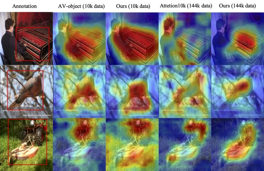
0.0~0.2        7.41%
                                                                                                      2.98%                   1
                                                                                          0.2~0.4
                                                                 28.5%                    0.4~0.6                             2
                                                                                 41.2%    0.6~0.8                             >2
                                                                                          0.8~1.0
                                                                 16.3%

                                                                         9.97%
                                                                                                                 89.6%

                                                                                   4.1%

                (a) VGG-SS benchmark examples                     (b) Bounding box areas            (c) Number of bounding boxes

Figure 3: VGG-SS Statistics. Figure 3a: Example VGG-SS images and annotations showing class diversity (humans,
animals, vehicles, tools etc.) Figure 3b: Distribution of bounding box areas in VGG-SS, the majority of boxes cover less
than 40% of the image area. Figure 3c shows the distribution of number of bounding boxes - roughly 10% of the test data is
challenging with more than one bounding box per image.

ification further cleans up the the test set, yielding a high-   with training sets consisting of image and audio pairs of
quality large-scale audio-visual benchmark — VGG-Sound           varying sizes, i.e. 10k, 144k and the full set.
Source (VGG-SS), which is 20 times larger than the exist-
ing one [31].                                                    5.2. Evaluation protocol
                                                                    In order to quantitatively evaluate the proposed ap-
 Stage               Goal               # Classes   # Videos     proach, we adopt the evaluation metrics used in [27, 31]:
                                                                 Consensus Intersection over Union (cIoU) and Area Under
   1     Automatic BBox Generation        309         15k
                                                                 Curve (AUC) are reported for each model on two test sets,
   2         Manual Annotation            260          8k
   3         Video Verification           220          5k
                                                                 as detailed next.
                                                                 Flickr SoundNet Testset: Following [18, 27, 31], we
Table 2: The number of classes and videos in VGG-SS after        report performance on the 250 annotated image-audio pairs
each annotation stage.                                           of the Flickr SoundNet benchmark. Every frame in this
                                                                 test set is accompanied by 20 seconds of audio, centered
5. Experiments                                                   around it, and is annotated with 3 separate bounding boxes
                                                                 indicating the location of the sound source, each performed
   In the following sections, we describe the datasets, eval-
                                                                 by a different annotator.
uation protocol and experimental details used to thoroughly
assess our method.                                               VGG-Sound Source (VGG-SS): We also re-implement
                                                                 and train several baselines on VGG-Sound and evaluate
5.1. Training Data                                               them on our proposed VGG-SS benchmark, described in
                                                                 section 4.
    For training our models, we consider two large-scale
audio-visual datasets, the widely used Flickr SoundNet           5.3. Implementation details
dataset and the recent VGG-Sound dataset, as detailed next.
Only the center frames of the raw videos are used for train-        As Flickr SoundNet consists of image-audio pairs, while
ing. Note, other frames e.g. (3/4 of the video) are tried for    VGG-Sound contains short video clips, when training on
training, no considerable performance change is observed.        the latter we select the middle frame of the video clip and
                                                                 extract a 3s audio segment around it to create an equivalent
Flickr SoundNet: This dataset was initially proposed in [3]
                                                                 image-audio pair. Audio inputs are 257 × 300 magnitude
and contains over 2 million unconstrained videos from
                                                                 spectrograms. The dimensions for the audio output from the
Flickr. For a fair comparison with recent work [18, 27, 31],
                                                                 audio encoder CNN is a 512D vector, which is max-pooled
we follow the same data splits, conducting self-supervised       from a feature map of 17 × 13 × 512, where 17 and 13 refer
training with subsets of 10k or 144k image and audio pairs.      to the frequency and time dimension respectively. For the
VGG-Sound: VGG-Sound was recently released with over             visual input, we resize the image to a 224 × 224 × 3 tensor
200k clips for 309 different sound categories. The dataset       without cropping. For both the visual and audio stream, we
is conveniently audio-visual, in the sense that the object       use a lightweight ResNet18 [16] as a backbone. Following
that emits sound is often visible in the corresponding video     the baselines [18, 27], we also pretrain the visual encoder
clip, which naturally suits the task considered in this paper.   on ImageNet. We use p = 0.65 and n = 0.4, τ = 0.03,
Again, to draw fair comparisons, we conduct experiments          that are picked by ablation study. All models are trained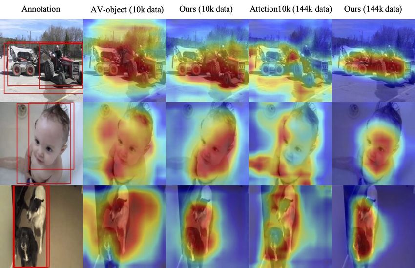
Model     Pos          Neg       Tri-map    CIoU     AUC
with the Adam optimizer using a learning rate of 10−4 and
a batch size of 256. During testing, we directly feed the full       a      X (0.6)        ×            ×       0.675    0.568
length audio spectrogram into the network.                           b      X (0.6)      X (0.6)        ×       0.667    0.544
                                                                     c      X (0.6)     X (0.45)        X       0.700    0.568
6. Results                                                           d      X (0.65)    X (0.45)        X       0.703    0.569
                                                                     e      X (0.65)    X (0.4)         X       0.719    0.582
   In the following sections, we first compare our results           f      X (0.7)     X (0.3)         X       0.687    0.563
with recent work on both Flickr SoundNet and VGG-SS
dataset in detail. Then we conduct an ablation analysis          Table 4: Ablation study. We investigate the effects of the
showing the importance of the hard negatives and the Tri-        hyper-parameters for defining positive and negative regions,
map in self-supervised audio-visual localization.                where the picked value is specified in the bracket.
6.1. Comparison on the Flickr SoundNet Test Set
                                                                             Method                CIoU     AUC
    In this section, we compare to recent approaches by
training on the same amount of data (using various differ-                   Attention10k [31]     0.185    0.302
ent datasets). As shown in Table 3, we first fix the train-                  AVobject [1]          0.297    0.357
ing set to be Flickr SoundNet with 10k training samples                      Ours                  0.344    0.382
and compare our method with [2, 15, 27]. Our approach            Table 5: Quantitative results on the VGG-SS testset. All
clearly outperforms the best previous methods by a sub-          models are trained on VGG-Sound 144k and tested on
stantial gap (0.546% vs. 0.582%). Second, we also train on       VGG-SS.
VGG-Sound using 10k random samples, which shows the
benefit of using VGG-Sound for training. Third, we switch
to a larger training set consisting of 144k samples, which       On introducing hard negative and Tri-map. While com-
gives us a further 5% improvement compared to the previ-         paring model a trained using only positives and model b
ous state-of-the-art method [18]. In order to tease apart the    adding negatives from the complementary region decreases
effect of various factors in our proposed approach, i.e. in-     performance slightly. This is because all the non-positive
troducing hard negative and using a Tri-map vs different         areas have been counted as negatives, whereas regions
training sets, i.e. Flickr144k vs. VGG-Sound144k, we con-        around the object are often hard to define. Therefore
duct an ablation study, as described next.                       deciding for all pixels whether they are positive or negative
                                                                 is problematic. Second, comparing model b and model c-f
 Method                Training set          CIoU     AUC        where some areas between positives and negatives are
                                                                 ignored during training by using the Tri-map, we obtain a
 Attention10k [31]     Flickr10k             0.436    0.449      large gain (around 2-4%), demonstrating the importance of
 CoarsetoFine [27]     Flickr10k             0.522    0.496      defining an “uncertain” region and allowing the model to
 AVObject [1]          Flickr10k             0.546    0.504      self-tune.
 Ours                  Flickr10k             0.582    0.525
 Ours                  VGG-Sound10k          0.618    0.536      On hyperparameters. we observe the model is generally
                                                                 robust to different set of hyper-parameters on defining the
 Attention10k [31]     Flickr144k            0.660    0.558      positive and negative regions, model-e (p = 0.65 and n =
 DMC [18]              Flickr144k            0.671    0.568      0.4) strives the best balance.
 Ours                  Flickr144k            0.699    0.573
 Ours                  VGG-Sound144k         0.719    0.582      6.3. Comparison on VGG-Sound Source
 Ours                  VGG-Sound Full        0.735    0.590
                                                                     In this section, we evaluate the models on the newly pro-
Table 3: Quantitative results on Flickr SoundNet testset. We     posed VGG-SS benchmark. As shown in Table 5, the CIoU
outperform all recent works using different training sets and    is reduced significantly for all models compared to the re-
number of training data.                                         sults in Table 3, showing that VGG-SS is a more diverse
                                                                 and challenging benchmark than Flickr SoundNet. How-
                                                                 ever, our proposed method still outperforms all other base-
6.2. Ablation Analysis                                           line methods by a large margin of around 5%.
   In this section, we train our method using the 144k-
                                                                 6.4. Qualitative results
samples training data from VGG-Sound and evaluate it on
the Flickr SoundNet test set, as shown in Table 4.                  In Figure 4, we threshold the heatmaps with different
                                                                 thresholds, e.g. p = 0.65 and n = 0.4 (same as the ones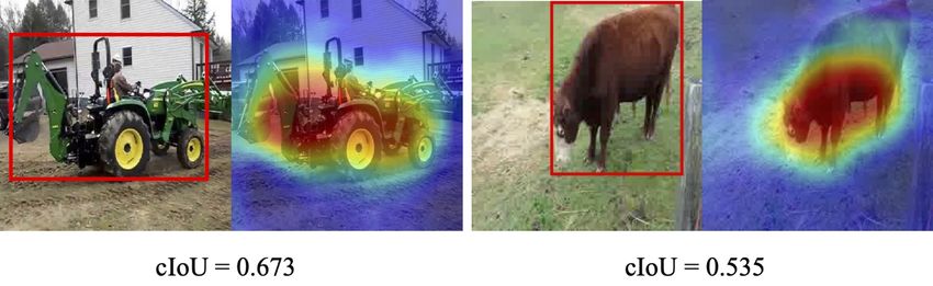
Figure 4: Example Tri-map visualisations. We show images, heatmaps and Tri-maps here. The Tri-map effectively identify
the objects and the uncertain region let the model only learn controlled hard negatives.

            (a) Visualisation on Flickr SoundNet testset                      (b) Visualisation on VGG-SS testset

Figure 5: Qualitative results for models trained on various methods and data amount. The first column shows annotation
overlaid on images, the following two column shows predictions trained on 10k data and the last tow column show predictions
trained on 144k data. Our method has no false positives in the predictions as the hard negatives are penalised in the training.

used during training). The objects and background are accu-
rately highlighted in the positive region and negative region           # training Data        Test class   CIoU    AUC
respectively, so that the model can learn proper amount of
                                                                        70k                  Heard 110      0.289   0.362
hard negatives. We visualize the prediction results in Fig-
                                                                        70k                Unheard 110      0.263   0.347
ure 5, and note that the proposed method presents much
cleaner heatmap outputs. This once again indicates the ben-       Table 6: Quantitative results on VGG-SS for unheard
efits of considering hard negatives during training.              classes. We vary the training set (classes) and keep the test-
                                                                  ing set fixed (subset of the VGG-SS).
6.5. Open Set Audio-visual Localization
   We have so far trained and tested our models on data
containing the same sound categories (closed set classifi-
cation). In this section we determine if our model trained        where for the heard split we also train the model on 70k
on heard/seen categories can generalize to classes that have      samples containing both old and new classes. The differ-
never been heard/seen before, i.e. to an open set scenario.       ence in performance is only 2%, which demonstrates the
To test this, we randomly sample 110 categories (seen/-           ability of our network to generalize to unheard or unseen
heard) from VGG-Sound for training, and evaluate our net-         categories. This is not surprising due to the similarity be-
work on another disjoint set of 110 unseen/unheard cate-          tween several categories. For example, if the training cor-
gories (for a full list please refer to appendix). We use         pus contains human speech, one would expect the model
roughly 70k samples for both heard and unheard classes.           to be capable of localizing human singing, as both classes
   Heard and unheard evaluations are shown in Table 6,            share semantic similarities in audio and visual features.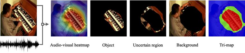
7. Conclusion                                                              Malik. Rich feature hierarchies for accurate object detection
                                                                           and semantic segmentation. In Proc. CVPR, 2014. 2
   We revisit the problem of unsupervised visual sound              [14]   Tengda Han, Weidi Xie, and Andrew Zisserman. Video rep-
source localization. For this task, we introduce a new large-              resentation learning by dense predictive coding. In Workshop
scale benchmark called VGG-Sound Source, which is more                     on Large Scale Holistic Video Understanding, ICCV, 2019.
challenging than existing ones such as Flickr SoundNet.                    4
We also suggest a simple, general and effective technique           [15]   David Harwath, Adria Recasens, Dı́dac Surı́s, Galen
that significantly boosts the performance of existing sound                Chuang, Antonio Torralba, and James Glass. Jointly dis-
                                                                           covering visual objects and spoken words from raw sensory
source locators, by explicitly mining for hard negative im-
                                                                           input. In Proc. ECCV, 2018. 1, 2, 4, 7
age locations in the same image that contains the sounding          [16]   Kaiming He, Xiangyu Zhang, Shaoqing Ren, and Jian Sun.
objecs. A careful implementation of this idea using Tri-                   Deep residual learning for image recognition. In Proc.
maps and differentiable thresholding allows us to signifi-                 CVPR, 2016. 6
cantly outperform the state of the art.                             [17]   John R. Hershey and Javier R. Movellan. Audio-vision: Lo-
                                                                           cating sounds via audio-visual synchrony. In NeurIPS, 1999.
Acknowledgements                                                           2
                                                                    [18]   Di Hu, Feiping Nie, and Xuelong Li. Deep multimodal clus-
   This work is supported by the UK EPSRC CDT                              tering for unsupervised audiovisual learning. In Proc. CVPR,
in Autonomous Intelligent Machines and Systems, the                        June 2019. 1, 2, 3, 6, 7
Oxford-Google DeepMind Graduate Scholarship, the                    [19]   Hamid Izadinia, Imran Saleemi, and Mubarak Shah. Mul-
Google PhD Fellowship, and EPSRC Programme Grants                          timodal analysis for identification and segmentation of
Seebibyte EP/M013774/1 and VisualAI EP/T028572/1.                          moving-sounding objects. IEEE Trans. Multimed., 2012. 2
                                                                    [20]   Naji Khosravan, Shervin Ardeshir, and Rohit Puri. On at-
                                                                           tention modules for audio-visual synchronization. In Proc.
                                                                           CVPR Workshop, 2019. 2
References                                                          [21]   Einat Kidron, Yoav Y Schechner, and Michael Elad. Pixels
 [1] Triantafyllos Afouras, Andrew Owens, Joon Son Chung, and              that sound. In Proc. CVPR, 2005. 2
     Andrew Zisserman. Self-supervised learning of audio-visual     [22]   Tsung-Yi Lin, Priya Goyal, Ross Girshick, Kaiming He, and
     objects from video. In Proc. ECCV, 2020. 1, 2, 3, 4, 7                Piotr Dollár. Focal loss for dense object detection. In Proc.
 [2] Relja Arandjelovic and Andrew Zisserman. Objects that                 ICCV, 2017. 2
     sound. In Proc. ECCV, 2017. 1, 2, 3, 4, 7                      [23]   Etienne Marcheret, Gerasimos Potamianos, Josef Vopicka,
 [3] Yusuf Aytar, Carl Vondrick, and Antonio Torralba. Sound-              and Vaibhava Goel. Detecting audio-visual synchrony using
     net: Learning sound representations from unlabeled video.             deep neural networks. In Proc. ICSA, 2015. 2
     In NeurIPS, 2016. 2, 6                                         [24]   Aaron van den Oord, Yazhe Li, and Oriol Vinyals. Repre-
 [4] Honglie Chen, Weidi Xie, Andrea Vedaldi, and Andrew Zis-              sentation learning with contrastive predictive coding. arXiv
     serman. VGG-Sound: A large-scale audio-visual dataset. In             preprint arXiv:1807.03748, 2018. 4
     Proc. ICASSP, 2020. 2, 5, 13                                   [25]   Andrew Owens and Alexei A. Efros. Audio-visual scene
 [5] Yung-Yu Chuang, Aseem Agarwala, Brian Curless, David H.               analysis with self-supervised multisensory features. In Proc.
     Salesin, and Richard Szeliski. Video matting of complex               ECCV, 2018. 1
     scenes. ACM Trans. Graph, 2002. 5                              [26]   Andrew Owens and Alexei A. Efros. Audio-visual scene
 [6] Joon Son Chung and Andrew Zisserman. Lip reading in the               analysis with self-supervised multisensory features. In Proc.
     wild. In Proc. ACCV, 2016. 2                                          ECCV, 2018. 2
 [7] Navneet Dalal and Bill Triggs. Histograms of oriented gra-     [27]   Rui Qian, Di Hu, Heinrich Dinkel, Mengyue Wu, Ning Xu,
     dients for human detection. In Proc. CVPR, 2005. 2                    and Weiyao Lin. Multiple sound sources localization from
 [8] Abhishek Dutta and Andrew Zisserman. The via annotation               coarse to fine. In Proc. ECCV, 2020. 2, 3, 6, 7
     software for images, audio and video. In Proc. ACMM, 2019.     [28]   Janani Ramaswamy and Sukhendu Das. See the sound, hear
     5, 13                                                                 the pixels. In Proc. WACV, 2020. 2
 [9] John W Fisher III, Trevor Darrell, William T Freeman, and      [29]   Shaoqing Ren, Kaiming He, Ross Girshick, and Jian Sun.
     Paul A Viola. Learning joint statistical models for audio-            Faster R-CNN: Towards real-time object detection with re-
     visual fusion and segregation. In NeurIPS, 2000. 2                    gion proposal networks. In NeurIPS, 2016. 2, 5
[10] Chuang Gan, Hang Zhao, Peihao Chen, David Cox, and An-         [30]   Andrew Rouditchenko, Hang Zhao, Chuang Gan, Josh Mc-
     tonio Torralba. Self-supervised moving vehicle tracking with          Dermott, and Antonio Torralba. Self-supervised audio-visual
     stereo sound. In Proc. ICCV, 2019. 2                                  co-segmentation. In Proc. ICASSP, 2019. 2
[11] Ruohan Gao and Kristen Grauman. 2.5d visual sound. In          [31]   Arda Senocak, Tae-Hyun Oh, Junsik Kim, Ming-Hsuan
     Proc. CVPR, 2019. 2                                                   Yang, and In So Kweon. Learning to localize sound source
[12] J Gemmeke, D Ellis, D Freedman, A Jansen, W Lawrence, C               in visual scenes. In Proc. CVPR, 2018. 1, 2, 3, 4, 5, 6, 7, 11
     Moore, M Plakal, and M Ritter. Audio Set: An ontology and      [32]   Abhinav Shrivastava, Abhinav Gupta, and Ross Girshick.
     human-labeled dataset for audio events. In Proc. ICASSP,              Training region-based object detectors with online hard ex-
     2017. 3                                                               ample mining. In Proc. CVPR, 2016. 2
[13] Ross Girshick, Jeff Donahue, Trevor Darrell, and Jitendra      [33]   Xin Tao, Hongyun Gao, Xiaoyong Shen, Jue Wang, and Ji-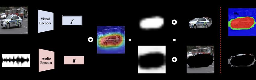
aya Jia. Scale-recurrent network for deep image deblurring.
       In Proc. CVPR, 2018. 5
[34]   Bart Thomee, David A Shamma, Gerald Friedland, Ben-
       jamin Elizalde, Karl Ni, Douglas Poland, Damian Borth, and
       Li-Jia Li. Yfcc100m: the new data in multimedia research.
       Commun. ACM, 2016. 2
[35]   Yapeng Tian, Jing Shi, Bochen Li, Zhiyao Duan, and Chen-
       liang Xu. Audio-visual event localization in unconstrained
       videos. In Proc. ECCV, 2018. 3
[36]   Paul Viola and Michael Jones. Robust real-time object de-
       tection. In Proc. SCTV Workshop, 2001. 2
[37]   Dingzeyu Li Yapeng Tian and Chenliang Xu. Unified mul-
       tisensory perception: Weakly-supervised audio-visual video
       parsing. In Proc. ECCV, 2020. 3
[38]   Hang Zhao, Chuang Gan, Wei-Chiu Ma, and Antonio Tor-
       ralba. The sound of motions. In Proc. ICCV, 2019. 2
[39]   Hang Zhao, Chuang Gan, Andrew Rouditchenko, Carl Von-
       drick, Josh McDermott, and Antonio Torralba. The sound of
       pixels. In Proc. ECCV, 2018. 2
Appendices
A. Evaluation metric
We follow the same evaluation metrics as in [31], and report consensus intersection over union (cIoU) and area under curve
(AUC). The Flickr Soundnet dataset contains 3 bounding box annotations from different human annotators. The bounding
box annotations are first converted into binary masks {bj }nj=1 where n is the number of bounding box annotations per image.
The final weighted ground truth mask is defined as:
n
X bj
g = min( , 1)
j=1
C
where C is a parameter meaning the minimum number of opinions to reach agreement. We choose C = 2, the same as [31].
Given the ground truth g and our prediction p, the cIoU is defined as
P
i∈A(τ ) gi
cIoU (τ ) = P P
i gi + i∈A(τ )−G 1
where i indicates the pixel index of the map, τ denotes the threshold to judge positiveness, A(τ ) = {i|pi > τ }, and
G = {i|gi > 0}. We follow [31], and use τ = 0.5. Example predictions and their cIoUs are shown in Figure 6.
Figure 6: Example predictions with calculated cIoU.
Since the cIoU is calculated for each testing image-audio pair, the success ratio is defined as number of successful samples
(cIoU greater than a threshold τ2 ) / total number of samples. The curve showing success ratio is plotted against the threshold
τ2 varied from 0 to 1 and the area under the curve is reported. The Pseudocode is shown in Algorithm 1.
Algorithm 1 Pseudocode of AUC calculation
# cIoUs : [cIoU_1,cIoU_2,...,cIoU_n]
x = [0.05 * i for i in range(21)]
for t in x: # Divide into 20 different thresholds
score.append(sum(cIoUs > t) / len(cIoUs))
AUC = calulcate_auc(x,score) # sklearn.metrics.auc
A.1. Tri-map visualisation
In addition to video examples, we show more image results of our Tri-maps in Figure 7.Figure 7: Tri-map visualization examples.
B. VGG-Sound Source (VGG-SS)
  We show more dataset examples, the full 220 class list of VGG-SS and the classes we removed from the original VGG-
Sound dataset [4] in this section.
B.1. VGG-SS annotation interface
   We show our manual annotation interface, LISA [8], in Figure 8. The example videos are from the class ‘Rapping’. The
‘Play’ button shows the 5s clip, and ‘Show region’ recenters to the key frame we want to annotate. We choose ‘Yes’ only if
we hear the correct sound, ‘No’ for the clips that do not contain the sound of class, and ‘Not Sure’ if the sound is not within
the 5s we choose (original video clip is 10s)

                                            Figure 8: LISA Annotation Interface

B.2. VGG-SS examples
   We randomly sample from images with 1 bounding box, 2 bounding boxes, and with more than 2 bounding boxes. We
show examples with 1 bounding box on the top 4 rows, examples with 2 bounding boxes on the following two rows, and
examples with more than 2 bounding boxes on the last row in Figure 9.
Figure 9: We show examples with 1 bounding box on the top 4 rows, examples with 2 bounding boxes on the following two rows, and examples with more than 2 bounding boxes on the last row.
Data amount
0 10 20 30 40
playing congas
playing djembe
parrot talking
tractor digging
dog growling
telephone bell ringing
driving snowmobile
cat hissing
cow lowing
reversing beeps
gibbon howling
playing violin, fiddle
playing steel guitar, slide guitar
playing acoustic guitar
helicopter
train whistling
playing cornet
wood thrush calling
snake hissing
bull bellowing
baltimore oriole calling
electric shaver, electric razor shaving
tap dancing
airplane flyby
playing tambourine
railroad car, train wagon
people giggling
playing oboe
people babbling
snake rattling
cat caterwauling
people eating noodle
people sniggering
driving motorcycle
playing bass guitar
pheasant crowing
child singing
black capped chickadee calling
alarm clock ringing
people slurping
engine accelerating, revving, vroom
disc scratching
tapping guitar
playing banjo
people hiccup
playing mandolin
playing erhu
fire truck siren
coyote howling
people belly laughing
ice cream truck, ice cream van
slot machine
male speech, man speaking
playing timbales
machine gun shooting
alligators, crocodiles hissing
magpie calling
car engine starting
playing glockenspiel
playing drum kit
playing harp
yodelling
canary calling
playing bongo
train wheels squealing
using sewing machines
elk bugling
people eating crisps
playing hammond organ
dog baying
fireworks banging
dog barking
owl hooting
dog bow-wow
subway, metro, underground
dinosaurs bellowing
popping popcorn
playing trumpet
missile launch
chicken clucking
lip smacking
lions roaring
female singing
cat meowing
chipmunk chirping
elephant trumpeting
playing accordion
bathroom ventilation fan running
playing bass drum
hedge trimmer running
turkey gobbling
car passing by
playing electronic organ
lathe spinning
playing guiro
pigeon, dove cooing
goat bleating
people sobbing
cuckoo bird calling
lawn mowing
woodpecker pecking tree
people booing
fox barking
children shouting
playing trombone
playing castanets
toilet flushing
barn swallow calling
playing harpsichord
crow cawing
playing ukulele
baby crying
waterfall burbling
wind chime
people coughing
playing theremin
typing on computer keyboard
female speech, woman speaking
driving buses
mynah bird singing
playing tympani
playing bassoon
bird chirping, tweeting
child speech, kid speaking
people whispering
playing cello
playing bugle
beat boxing
people marching
people cheering
baby laughter
motorboat, speedboat acceleration
race car, auto racing
chainsawing trees
playing harmonica
warbler chirping
chicken crowing
skidding
playing didgeridoo
opening or closing car electric windows
dog howling
electric grinder grinding
airplane
lions growling
squishing water
eletric blender running
donkey, ass braying
playing washboard
playing piano
sharpen knife
playing flute
people sneezing
people eating apple
playing electric guitar
playing table tennis
people burping
vacuum cleaner cleaning floors
singing choir
male singing
police car (siren)
playing double bass
playing shofar
sea lion barking
cat growling
playing french horn
playing clarinet
air horn
blowtorch igniting
hair dryer drying
cattle mooing
people whistling
skateboarding
opening or closing drawers
cat purring
people screaming
eagle screaming
sheep bleating
playing saxophone
chinchilla barking
forging swords
people humming
horse clip-clop
cheetah chirrup
chimpanzee pant-hooting
car engine idling
playing zither
ocean burbling
church bell ringing
cap gun shooting
cattle, bovinae cowbell
typing on typewriter
people finger snapping
rowboat, canoe, kayak rowing
francolin calling
penguins braying
cricket chirping
civil defense siren
bird wings flapping
smoke detector beeping
bird squawking
people shuffling
playing steelpan
lighting firecrackers
otter growling
train horning
air conditioning noise
people crowd
singing bowl
people battle cry
playing cymbal
people nose blowing
whale calling
mouse squeaking
playing snare drum
orchestra
playing gong
fly, housefly buzzing
dog whimpering
splashing water
car engine knocking
people gargling
Figure 10: VGG-SS benchmark per class statistics.B.3. VGG-SS class list 30. snake rattling (34)
We show a bar chart of per-class frequencies for the 31. cat caterwauling (33)
VGG-SS testset in Figure 10. The full list below is shown
in the format of index. class name (number of clips in the 32. people eating noodle (33)
class).
33. people sniggering (32)
1. playing congas (45)
34. driving motorcycle (32)
2. playing djembe (45) 35. playing bass guitar (32)
3. parrot talking (43) 36. pheasant crowing (32)
4. tractor digging (42) 37. child singing (32)
5. dog growling (41) 38. black capped chickadee calling (32)
6. telephone bell ringing (40) 39. alarm clock ringing (31)
7. driving snowmobile (39) 40. people slurping (31)
8. cat hissing (39) 41. engine accelerating, revving, vroom (31)
9. cow lowing (39) 42. disc scratching (31)
10. reversing beeps (38) 43. tapping guitar (31)
11. gibbon howling (38) 44. playing banjo (31)
12. playing violin, fiddle (38) 45. people hiccup (31)
13. playing steel guitar, slide guitar (38) 46. playing mandolin (31)
14. playing acoustic guitar (36) 47. playing erhu (31)
15. helicopter (36) 48. fire truck siren (31)
16. train whistling (36) 49. coyote howling (31)
17. playing cornet (36) 50. people belly laughing (31)
18. wood thrush calling (35) 51. ice cream truck, ice cream van (30)
19. snake hissing (35) 52. slot machine (30)
20. bull bellowing (35) 53. male speech, man speaking (30)
21. baltimore oriole calling (35) 54. playing timbales (30)
22. electric shaver, electric razor shaving (35) 55. machine gun shooting (29)
23. tap dancing (35) 56. alligators, crocodiles hissing (29)
24. airplane flyby (35) 57. magpie calling (29)
25. playing tambourine (35) 58. car engine starting (29)
26. railroad car, train wagon (35) 59. playing glockenspiel (29)
27. people giggling (34) 60. playing drum kit (29)
28. playing oboe (34) 61. playing harp (28)
29. people babbling (34) 62. yodelling (28)63. canary calling (28) 96. pigeon, dove cooing (24) 64. playing bongo (28) 97. goat bleating (24) 65. train wheels squealing (28) 98. people sobbing (24) 66. using sewing machines (28) 99. cuckoo bird calling (23) 67. elk bugling (28) 100. lawn mowing (23) 68. people eating crisps (28) 101. woodpecker pecking tree (23) 69. playing hammond organ (27) 102. people booing (23) 70. dog baying (27) 103. fox barking (23) 71. fireworks banging (27) 104. children shouting (23) 72. dog barking (27) 105. playing trombone (23) 73. owl hooting (27) 106. playing castanets (22) 74. dog bow-wow (27) 107. toilet flushing (22) 75. subway, metro, underground (27) 108. barn swallow calling (22) 76. dinosaurs bellowing (26) 109. playing harpsichord (22) 77. popping popcorn (26) 110. crow cawing (22) 78. playing trumpet (26) 111. playing ukulele (22) 79. missile launch (26) 112. baby crying (22) 80. chicken clucking (26) 113. waterfall burbling (22) 81. lip smacking (26) 114. wind chime (22) 82. lions roaring (26) 115. people coughing (21) 83. female singing (26) 116. playing theremin (21) 84. cat meowing (25) 117. typing on computer keyboard (21) 85. chipmunk chirping (25) 118. female speech, woman speaking (21) 86. elephant trumpeting (25) 119. driving buses (21) 87. playing accordion (25) 120. mynah bird singing (21) 88. bathroom ventilation fan running (25) 121. playing tympani (21) 89. playing bass drum (25) 122. playing bassoon (21) 90. hedge trimmer running (25) 123. bird chirping, tweeting (21) 91. turkey gobbling (25) 124. child speech, kid speaking (21) 92. car passing by (24) 125. people whispering (21) 93. playing electronic organ (24) 126. playing cello (21) 94. lathe spinning (24) 127. playing bugle (21) 95. playing guiro (24) 128. beat boxing (21)
129. people marching (21)                           162. playing shofar (18)
130. people cheering (20)                           163. sea lion barking (18)
131. baby laughter (20)                             164. cat growling (17)
132. motorboat, speedboat acceleration (20)         165. playing french horn (17)
133. race car, auto racing (20)                     166. playing clarinet (17)
134. chainsawing trees (20)                         167. air horn (17)
135. playing harmonica (20)                         168. blowtorch igniting (16)
136. warbler chirping (20)                          169. hair dryer drying (16)
137. chicken crowing (20)                           170. cattle mooing (16)
138. skidding (20)                                  171. people whistling (16)
139. playing didgeridoo (20)                        172. skateboarding (16)
140. opening or closing car electric windows (20)   173. opening or closing drawers (16)
141. dog howling (20)                               174. cat purring (16)
142. electric grinder grinding (20)                 175. people screaming (16)
143. airplane (20)                                  176. eagle screaming (16)
144. lions growling (20)                            177. sheep bleating (16)
145. squishing water (20)                           178. playing saxophone (16)
146. eletric blender running (20)                   179. chinchilla barking (16)
147. donkey, ass braying (19)                       180. forging swords (16)
148. playing washboard (19)                         181. people humming (15)
149. playing piano (19)                             182. horse clip-clop (15)
150. sharpen knife (19)                             183. cheetah chirrup (15)
151. playing flute (19)                             184. chimpanzee pant-hooting (15)
152. people sneezing (19)                           185. car engine idling (15)
153. people eating apple (19)                       186. playing zither (15)
154. playing electric guitar (19)                   187. ocean burbling (15)
155. playing table tennis (19)                      188. church bell ringing (15)
156. people burping (19)                            189. cap gun shooting (15)
157. vacuum cleaner cleaning floors (19)            190. cattle, bovinae cowbell (15)
158. singing choir (19)                             191. typing on typewriter (14)
159. male singing (18)                              192. people finger snapping (14)
160. police car (siren) (18)                        193. rowboat, canoe, kayak rowing (14)
161. playing double bass (18)                       194. francolin calling (14)
195. penguins braying (14)         B.4. Removed classes
                                    1. running electric fan
196. cricket chirping (13)
                                    2. mouse clicking
197. civil defense siren (13)
                                    3. people eating
198. bird wings flapping (13)       4. people clapping
199. smoke detector beeping (13)    5. roller coaster running

200. bird squawking (13)            6. cell phone buzzing
                                    7. basketball bounce
201. people shuffling (13)
                                    8. playing timpani
202. playing steelpan (12)
                                    9. people running
203. lighting firecrackers (12)    10. firing muskets

204. otter growling (12)           11. door slamming
                                   12. hammering nails
205. train horning (12)
                                   13. chopping wood
206. air conditioning noise (12)
                                   14. striking bowling
207. people crowd (12)             15. bowling impact

208. singing bowl (11)             16. ripping paper
                                   17. baby babbling
209. people battle cry (11)
                                   18. playing hockey
210. playing cymbal (11)
                                   19. swimming
211. people nose blowing (11)
                                   20. hail
212. whale calling (11)            21. people slapping

213. mouse squeaking (11)          22. wind rustling leaves
                                   23. sea waves
214. playing snare drum (11)
                                   24. heart sounds, heartbeat
215. orchestra (10)
                                   25. raining
216. playing gong (10)             26. rope skipping

217. fly, housefly buzzing (10)    27. stream burbling
                                   28. playing badminton
218. dog whimpering (10)
                                   29. striking pool
219. splashing water (10)
                                   30. wind noise
220. car engine knocking (10)      31. bouncing on trampoline
221. people gargling (10)          32. thunder
33. ice cracking 34. shot football 35. playing squash 36. scuba diving 37. cupboard opening or closing 38. fire crackling 39. playing volleyball 40. golf driving 41. sloshing water 42. sliding door 43. playing tennis 44. footsteps on snow 45. people farting 46. playing marimba, xylophone 47. foghorn 48. tornado roaring 49. playing lacrosse
You can also read