Margin Trading and Leverage Management - WORKING PAPER NO. 2021-29 Jiangze Bian, Zhi Da, Zhiguo He, Dong Lou, Kelly Shue, and Hao Zhou - The ...
←
→
Page content transcription
If your browser does not render page correctly, please read the page content below
WORKING PAPER · NO. 2021-29

Margin Trading and Leverage Management
Jiangze Bian, Zhi Da, Zhiguo He, Dong Lou, Kelly Shue, and Hao Zhou
MARCH 2021

                                                                      5757 S. University Ave.
                                                                          Chicago, IL 60637
                                                                         Main: 773.702.5599
                                                                           bfi.uchicago.edu
Margin Trading and Leverage Management∗
Jiangze Bian, Zhi Da, Zhiguo He, Dong Lou, Kelly Shue, Hao Zhou
This Draft: March 2021
Abstract
We use granular data covering regulated (brokerage-financed) and unregulated (shadow-financed)
margin trading during the 2015 market turmoil in China to provide the first systematic analysis
of margin investors’ characteristics, leverage management policies, and liquidation choices. We
show that leverage constraints induced substantial forced and preemptive sales, and leverage
and cash management differed substantially across investor and account types. We explore the
relation between margin trading and shock propagation, and show that China’s price limit rule
led to unintended contagion across stocks. Compared to brokerage investors, shadow investors
were closer to their leverage constraints, and played a more significant role in transmitting
shocks across stocks.
Keywords: margin trading, leverage management, liquidation policy, contagion
∗
Bian: University of International Business and Economics, jiangzebian@uibe.edu.cn. Da: University of Notre
Dame, zda@nd.edu. He: University of Chicago and NBER, zhiguo.he@chicagobooth.edu. Lou: London School of
Economics and CEPR, d.lou@lse.ac.uk. Shue: Yale University and NBER, kelly.shue@yale.edu. Zhou: PBC School
of Finance, Tsinghua University, zhouh@pbcsf.tsinghua.edu.cn. This paper subsumes two previous working papers:
“Leverage-Induced Fire Sales and Stock Market Crashes” by Bian, He, Shue and Zhou, and “Leverage Networks
and Market Contagion” by Bian, Da, Lou and Zhou. We are grateful to participants at numerous meetings and
seminars for helpful comments, and to Yiran Fan, Daniel Huang, Jianglong Wu, Hong Xiang, Xiao Zhang for their
excellent research assistance. Bian acknowledges financial support from the National Natural Science Foundation of
China (Project No. 72073027). He acknowledges financial support from the Fama-Miller Center at the University of
Chicago, Booth School of Business. Lou acknowledges funding from the Paul Woolley Center at the London School
of Economics. All remaining errors are our own.1 Introduction
Investors can use margin trading—the practice of borrowing against the securities they hold—
to amplify returns. In standard asset pricing models, as well as in practice, investors lend to and
borrow from one another to clear both the risk-free and risky securities markets. A well-functioning
lending-borrowing market is therefore crucial to a healthy financial system. Despite the apparent
importance, there is little empirical evidence on investors’ margin trading decisions, mainly due
to a lack of granular data. For example, we know little about the characteristics of investors that
choose to use margin borrowing, margin investors’ leverage- and liquidity-management policies
(specifically, how these policies vary with investor demographics and trading experiences, as well
as the regulatory environment and advancement of FinTech-driven shadow financing), and finally,
the asset pricing implications of margin-induced trading.
In this paper, we provide novel analysis of investor margin trading behavior using detailed
account-level data in China that tracks hundreds of thousands of margin investors’ borrowing and
trading activities. The Chinese economy and its financial markets have experienced tremendous
growth in the last three decades.1 With a total market capitalization of roughly one-third of that
of the US, the Chinese stock market is now the second largest in the world. Our data cover an
extraordinary three-month period of the Chinese stock market, May to July 2015: the market grew
steadily in the spring of 2015, continued with a strong run-up from May to mid-June, and then
experienced a dramatic crash in mid-June that wiped out nearly 30% of the market value by the
end of July 2015.2
Individual retail investors are the dominant players in the Chinese stock market and are the
main users of margin trading.3 Our data include two types of margin trading systems: brokerage-
financed and shadow-financed margin accounts. Both margin trading systems grew rapidly in
popularity in early 2015. The brokerage-financed margin system, which allows retail investors to
obtain credit from their brokerage firms, is tightly regulated by the China Securities Regulatory
Commission (CSRC). For instance, investors must be sufficiently wealthy and experienced to qualify
for brokerage financing. Further, the CSRC imposes a market-wide maximum level of leverage—the
Pingcang Line—beyond which the account is taken over by the lending broker, triggering forced
liquidation.4
In contrast, the shadow-financed margin system, aided by China’s burgeoning FinTech industry,
falls in a regulatory grey area. Shadow-financing is largely unregulated by the CSRC, and lenders
1
For an informative reading, see Carpenter and Whitelaw (2017) and Allen et al. (2020).
2
Excessive leverage and the subsequent leverage-induced fire sales are considered to be contributing factors to
many past financial crises. A prominent example is the US stock market crash of 1929 (Schwert (1989), Galbraith
(2009)). Other significant examples of deleveraging and market crashes include the US housing crisis which led to
the 2007/08 global financial crisis (Mian et al. (2013)), the “Quant Meltdown” of August 2007 (Khandani and Lo
(2011)), and the Chinese stock market crash in the summer of 2015 (which will be the focus of this paper).
3
Trading by retail investors accounts for over 85% of total trading volume, according to Shanghai Stock Exchange
Annual Statistics 2015.
4
The maximum leverage or Pingcang Line corresponds to the reciprocal of the maintenance margin in the U.S.
market. “Pingcang” in Chinese means “forced settlement” by creditors.
1generally do not impose restrictions on borrower wealth, trading experience, or financial literacy.
There is no regulatory maximum Pingcang Line for shadow-financed margin accounts. Instead,
the maximum leverage limits are market outcomes determined by bilateral negotiations between
borrowers and lenders. We find that shadow accounts have significantly higher leverage limits
and realized leverage than their brokerage counterparts; for example, the average leverage (=
assets/equity) is 6.9 for shadow-financed margin accounts and only 1.4 for brokerage-financed
accounts.
We begin our analysis by examining the types of investors that are more likely to use margin
borrowing (the extensive margin), and have higher initial leverage conditional on using margin (the
intensive margin). Consistent with the idea that heterogeneous risk preferences determine margin
trading, we find that more leveraged traders are less experienced, more active, male, and take on
higher portfolio risk.
We next study the relation between investors’ margin borrowing and their trading and cash-
management decisions. For each account-date, we compute its “distance-to-margin-call,” the
difference between the account’s leverage (assets/equity) and its Pingcang Line, scaled by the asset
volatility. In other words, “distance-to-margin-call” measures the number of standard deviations
of downward movements in asset values necessary to push the account’s leverage to its Pingcang
Line. Similar to distance-to-default measures in Merton-style models, the distance-to-margin-call
in our setting captures the risk of a margin account hitting its Pingcang Line and consequently
being taken over by its creditor (i.e., when the distance-to-margin-call hits zero).
In the theoretical literature, static models such as Brunnermeier and Pedersen (2009) and
Geanakoplos (2010) predict that levered investors and their creditors engage in fire sales only when
accounts hit the Pingcang Line. However, investors may engage in preemptive selling prior to hitting
the Pingcang Line for several reasons. In a dynamic setting such as Garleanu and Pedersen (2011),
forward-looking investors sell before hitting the leverage constraint, because they anticipate that the
controlling creditor will liquidate stock holdings with some fire-sale cost. Investors’ precautionary
selling prior to hitting the Pingcang Line can also be explained by runs in financial markets, as
illustrated by Bernardo and Welch (2004).5 Finally, investors may engage in precautionary sales
because they fear (rationally or irrationally) that creditors, once they seize control, will sell assets
while their prices are temporarily depressed.
We find strong empirical support for both forced and preemptive margin-induced trading in
our data. Specifically, after controlling for account- and stock-date- fixed effects, we show that net
buying is positively related to the account’s distance-to-margin-call (which we label “Z”), and to
recent changes in this distance (which we label “Z-shocks” and is driven by recent account returns).
For example, margin accounts with Z ∈ (0, 1] (i.e., accounts that would hit the Pingcang Line after
a one standard deviation negative shock) sell 18.4% of their risky holdings on that day, relative to
5
In Bernardo and Welch (2004), liquidity runs are not caused by liquidity shocks per se, but by the fear of future
liquidity shocks. This is in complement to the bank-run mechanism in Diamond and Dybvig (1983), Goldstein and
Pauzner (2005) and recently He and Xiong (2012)).
2non-levered margin accounts. The coefficients on Z and Z-shocks are larger for female investors
and depend on trading restrictions faced by margin investors (to be explained shortly).
It is worth noting that the strong relation between investors’ net buying and both the level and
change in the distance-to-margin-call can be attributed to two potential mechanisms: (1) leverage
constraints, i.e., forced and preemptive sales that occur when account leverage approaches its
leverage limit; and (2) a portfolio rebalancing motive that leads risk-averse investors with a target
leverage level to adjust leverage after a drop or increase in asset value (which leads to a mechanical
increase or decrease in leverage, respectively). Thus, leverage-induced sales in our setting should
be viewed as a combination of these two widely-accepted economic forces: one that consists of
preemptive and/or forced sales due to tightening leverage constraints and the other driven by a
rebalancing motive that would occur even in the absence of Pingcang Lines.
While we believe that both forces play a role in our setting, we provide further evidence for
the importance of the leverage constraints channel. First, we compare investors’ responses to
positive and negative Z-shocks. A simple model of a portfolio rebalancing motive predicts that
investors should react to both positive and negative Z-shocks. Instead, we find that investors sell
aggressively in response to negative Z-shocks but do not buy significantly in response to positive
Z-shocks. This behavior is consistent with the idea that investors face stronger incentives to adjust
their risky holdings when the leverage constraint tightens than when it loosens. We also present
additional tests in Section 4.3.4 to rule in the role of forced sales and leverage constraints. These
tests exploit the granularity of our shadow account data, and use variation in Pingcang Lines across
accounts to identify a leverage constraint effect.
Although both brokerage-financed and shadow-financed margin accounts reduce their risky
holdings in response to tightening leverage constraints, the two groups behave very differently
in their cash and liability management decisions. Brokerage-financed margin accounts use sales
proceeds to pay down debt immediately. In contrast, shadow-financed margin accounts keep most
of the sales proceeds as cash instead of paying down debt. One possible explanation for this
intriguing difference is that the brokerage margin system is more “rule-based,” while the shadow
system is more “discretion-based.” Because brokerage firms allow any account in good standing to
increase or reduce leverage at any time, maintaining a cash balance while carrying margin debt is
suboptimal given the high interest cost of margin loans. In the shadow margin system, however,
each new borrowing request must be approved by the lender. Consequently, despite the higher
interest rates for shadow accounts, shadow-financed margin investors worry about future financing
needs, and therefore choose to hoard cash today. In other words, frictions in the shadow margin
system may lead investors to hoard “ borrowed” cash, thereby contributing to the persistently high
leverage.
We also uncover an important unintended consequence of trading restrictions imposed by the
government. In Chinese markets, a stock cannot be bought or sold if it is suspended from trading, or
if the stock hits its daily upper or lower price limit, equal to 110 or 90% of its previous day’s closing
3price, respectively. We find that a stock is sold in larger proportions (in response to changes in
distance-to-margin-call) by margin accounts whose other holdings cannot be traded due to trading
restrictions. Thus, trading restrictions on stocks that have declined in value lead to liquidation of
other stocks held by leveraged accounts, resulting in contagion from unhealthy to healthy stocks.
As a natural extension, we also analyze margin investors’ liquidation choice more generally,
by examining the types of stocks that margin investors are more likely to buy or sell in response
to changes in the distance-to-margin-call. Conceptually, liquidation choice can be affected by a
number of stock and account characteristics, including riskiness, liquidity, and position size. We
conduct panel regressions of investors’ trading activity in individual stocks on various stock/position
characteristics interacted with account-level distance-to-margin-call shocks. We find that margin
investors are more likely to liquidate stocks that are more expensive (relative to book value), larger,
and more liquid, when faced with tightening leverage constraints. Brokerage margin investors also
exhibit behavior consistent with a disposition effect, in which they are more willing to sell stocks
with positive recent returns.
Finally, we study contagion across stocks with common ownership by margin accounts. The idea
is that an initial reduction in account value tightens the leverage constraint, leading to additional
selling and hence even lower prices. Extending this well-established fire-sale mechanism to a setting
with multiple assets, we conjecture that if investors downsize all their holdings—including those
that have not gone down in value and thus have little to do with the initial tightening of the leverage
constraint—in reaction to negative return shocks, leverage-induced trading can generate contagion
across assets that are linked through common ownership by levered investors.
We examine this shock propagation mechanism by constructing a stock-level measure of “margin-
account linked portfolio returns” (M LP R) based on a theoretically-motivated framework. Specifically,
M LP R for a stock is defined as the weighted-average daily return of all margin accounts holding
the stock on a particular day, after removing the stock’s own contribution to each account’s return
(so as to isolate the effect of contagion). Importantly, the weights are based on a function of the
distance-to-margin-call of each account, to reflect our earlier finding that leverage-induced selling
depends on how close the account is to hitting its leverage constraint.
We indeed find that M LP R forecasts the corresponding stock’s next-day return. While this
result is consistent with transmission of shocks via leverage-induced trading, it is also consistent
with a key alternative explanation. Margin traders do not choose stock holdings randomly, and
they may hold related stocks that move together for other reasons.
We address this potential alternative explanation in several ways. First, we control for observable
stock characteristics and past return patterns that could lead to stocks to move together. Second,
we show that M LP R only predicts stock returns during downturns. This asymmetric response does
not match a simple related holdings story in which related stocks should experience both positive
and negative comovement. We also show that selling restrictions transmit negative return shocks
from unhealthy stocks (which cannot be sold) to healthier stocks (which are the only stocks that
4leveraged investors can sell). We construct two M LP R measures for each stock based on accounts
with high and low selling restrictions for other holdings, and show that M LP R with high selling
restrictions is associated with much stronger return predictability.
We also control for a related holdings effect by constructing “non-margin-account linked portfolio
returns” (N M LP R) using non-margin brokerage accounts that are similar to margin accounts in
size and trading volume. Empirically, we find that N M LP R does not predict future returns
and controlling for N M LP R does not change the predictive power of M LP R. To the extent that
matched non-margin accounts choose to hold related stocks in a similar fashion to margin accounts,
controlling for N M LP R helps tease out true contagion due to leverage constraints. In a related test,
we show that M LP R constructed using only shadow accounts predicts returns more strongly than
M LP R constructed using only brokerage accounts, despite brokerage accounts holding substantially
greater total asset value. This suggests shadow margin traders played a more significant role in
transmitting shocks via the leverage network, in line with the fact that shadow accounts were
far more leveraged relative to their leverage limits and thus experienced greater leverage-induced
selling. Finally, we show that the return impact of M LP R reverts in approximately one month,
consistent with M LP R being a non-fundamental shock.
In summary, our analyses of shock propagation provide evidence of a) an asymmetry between
market booms and busts, b) a sharp contrast between the price impact of common holdings of
margin and non-margin accounts, and c) a similar contrast between the price impact of common
holdings by constrained and unconstrained margin accounts, and d) an initial price effect followed
by a gradual return reversal. This set of results on return predictability, when taken as a whole,
helps alleviate the concern that our documented contagion pattern is due to correlated fundamental
shocks to commonly-held stocks.
Related literature Our paper contributes to the literature on the role of funding constraints in
asset pricing. Theoretical contributions such as Kyle and Xiong (2001), Gromb and Vayanos (2002),
Danielsson et al. (2002), Geanakoplos (2010), Fostel and Geanakoplos (2008), Brunnermeier and
Pedersen (2009), and Garleanu and Pedersen (2011) help academics and policymakers understand
the linkages between funding constraints and asset prices, especially in the aftermath of the
recent global financial crisis.6 There is also an empirical literature that connects various funding
constraints to asset prices. Hardouvelis (1990) finds that a tighter margin requirement is associated
with lower volatility in the US stock market. This is consistent with an underlying mechanism in
which tighter margin requirements discourage optimistic investors from taking speculative positions
(this mechanism may also apply to retail investors in the Chinese stock market). Hardouvelis and
Theodossiou (2002) further show that the relation between margin requirements and volatility only
holds in bull and normal markets. This finding points to the potential benefit of margin credit,
6
Another important strand of the literature explores heterogeneous portfolio constraints in a general equilibrium
asset pricing framework and its macroeconomic implications, which features an “equity constraint,” for instance,
Basak and Cuoco (1998); He and Krishnamurthy (2013); Brunnermeier and Sannikov (2014).
5in that it essentially relaxes funding constraints. Closely related to our paper is Kahraman and
Tookes (2017). By comparing marginable vs. otherwise similar non-marginable stocks in the Indian
market, Kahraman and Tookes (2017) analyze the impact of margin trading on stock liquidity as
well as commonality in liquidity. Our detailed account-level data allow us to precisely measure how
each account manages its leverage ratio (which is not available in the Indian setting) and examine
its impact on account trading, and ultimately stock returns.7 Chen et al. (2021) estimates the
value of marginability by studying Chinese corporate bond markets where bonds with identical
fundamentals are simultaneously traded on two segmented markets that feature different rules for
repo transactions.
Our paper is also related to a large literature on fire sales in various asset markets including the
stock market, housing market, derivatives market, and even markets for real assets (e.g., aircraft).
A seminal paper by Shleifer and Vishny (1992) argues that asset fire sales are possible when
financial distress clusters at the industry level, as the natural buyers of the asset are financially
constrained. Pulvino (1998) tests this theory by studying commercial aircraft transactions initiated
by (capital) constrained versus unconstrained airlines, and Campbell et al. (2011) document fire
sales in local housing market due to events such as foreclosures. In the context of financial markets,
Coval and Stafford (2007) show the existence of fire sales by studying open-end mutual fund
redemptions and the associated non-information-driven sales; Mitchell et al. (2007) investigate
the price reaction of convertible bonds around hedge fund redemptions; Ellul et al. (2011) show
that downgrades of corporate bonds may induce regulation-driven selling by insurance companies.
Recently, fire sales have been documented in the market for residential mortgage-backed securities
(Merrill et al. (2016)) and minority equity stakes in publicly-listed third parties (Dinc et al. (2017)).
We contribute to this literature by showing how leverage constraints cause investors to sell assets,
thereby impacting prices. We also use a variety of techniques to rule in a direct leverage constraint
effect, as distinct from a rebalancing channel.
Our paper also complements the recent literature on excess volatility and comovement induced
by common institutional ownership (e.g., Greenwood and Thesmar (2011); Lou (2012); Anton and
Polk (2014)). These studies focus on common holdings by non-margin investors such as mutual
funds. They also focus on transmission via the well-known flow-performance relation. Our paper
contributes to this literature by highlighting the role of leverage, in particular leverage-induced
selling, in driving asset returns.A unique feature of our leverage channel is that its return effect
is asymmetric (Hardouvelis and Theodossiou (2015)); using the recent boom-bust episode in the
Chinese stock market as our testing ground, we show that the leverage-induced return pattern is
present only in market downturns.
Our analysis of unique shadow margin data also offers insight into how investors behave when
7
The instrument used by Kahraman and Tookes (2017)—that stocks are periodically added to/deleted from the
marginable list (a featured also shared by the Chinese market)—is invalid in our setting. This is because a) virtually
all margin investors in our sample hold both marginable and non-marginable stocks (a margin investor can use his
own money to buy non-marginable stocks and borrowed money to buy marginable stocks), and b) this rule does not
apply to shadow-financed margin accounts.
6new financial innovations relax leverage constraints ahead of regulation. In our case, developments
in FinTech spurred rapid growth of unregulated margin borrowing (see e.g., Chen et al. (2018b);
Chen et al. (2020); and Gambacorta et al. (2020)). While the available technology obviously
differed, our modern Chinese setting can also be viewed as providing a parallel for the US stock
market crash of 1929 (see e.g., Schwert (1989)). Leverage for stock market margin trading was also
unregulated in the US at the time. Margin credit rose from around 12% of NYSE market value in
1917 to around 20% in 1929. In October 1929, investors began facing margin calls. As investors
quickly sold assets to delever their positions, the Dow Jones Industrial Average experienced a
record loss of 13% on October 28, 1929. As a consequence, regulation of margin requirements
were introduced through the Securities and Exchange Act of 1934. The rationale for margin
requirements at the time was precisely that credit-financed speculation in the stock market may
lead to excessive price movements through a “pyramiding-depyramiding” process. It is conceivable
that other developing markets may face similar issues.
Finally, given the increasing importance of the Chinese market in the world economy (second
only to the U.S.), understanding the boom and bust episode in 2015 is an informative exercise in
and of itself. Taking advantage of our novel account-level data, we provide the first comprehensive
evidence of how margin-induced trading may affect asset prices in the cross-section during this
extraordinary episode. Focusing on the initial boom of the same episode in China, Hansman et al.
(2018) provide evidence that margin debt indeed helped fuel the initial rally in the Chinese stock
market, a result that nicely complements ours. They do not, however, study account-level behavior
nor the contagion effect as we do. Liao et al. (2020) study the interplay between extrapolative beliefs
and the disposition effect using account-level trading records during the same 2014-15 Chinese stock
market bubble; they do not, however, analyze the behavior of margin investors during this episode.
2 Institutional Background and Data Sample
2.1 Institutional Background
Our analysis exploits account-level margin trading data in the Chinese stock market covering the
period May 1st to July 31st, 2015. We provide details of the institutional background in this
section.
2.1.1 Margin trading in the Chinese stock market in 2015
The Chinese stock market experienced a large run-up in the first half of 2015, followed by a dramatic
crash in mid-2015. The Shanghai Stock Exchange (SSE) Composite Index started at around 3100
in January 2015, peaked at 5166 in mid-June, and took a nose dive to 3663 at the end of July. It
is widely believed that high levels of margin borrowing and the subsequent leverage-induced fire
sales played a role in the market run-up and crash.
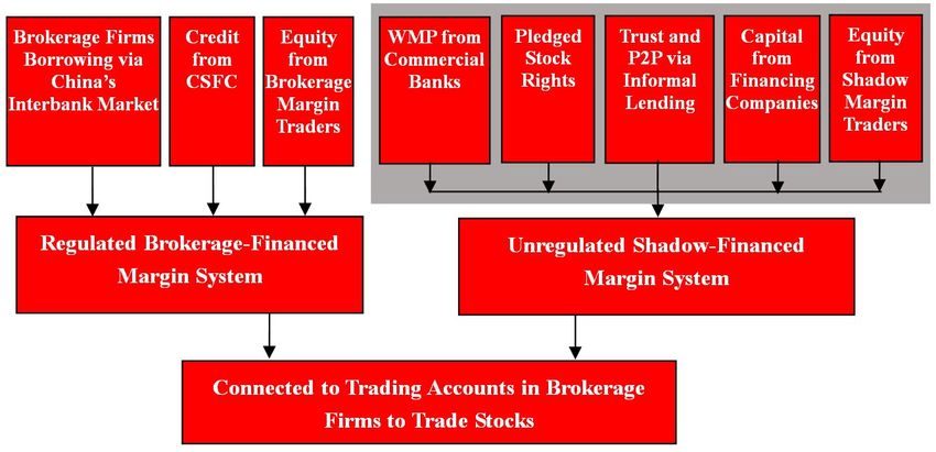
7There were two types of margin trading systems in China during this time. One is brokerage-
financed and the other is shadow-financed. Figure 1 shows the structures and funding sources of
the two margin trading systems.8 Both systems came into existence in 2010, and thrived after 2014
alongside a surge in the Chinese stock market. Throughout the paper, whenever there is no risk
of confusion, we use brokerage (shadow) accounts to refer to brokerage-financed (shadow-financed)
margin accounts.
2.1.2 Brokerage-financed margin accounts
Margin trading through brokerage firms was introduced in 2010, but saw little utilization until
mid-2014, at which point brokerage-financed margin trading started to grow exponentially. The
total debt held by brokerage-financed margin accounts stood at 0.4 trillion Yuan in June 2014, and
more than quintupled to 2.2 trillion Yuan after one year.9 This amounted to approximately 3-4%
of the total market capitalization of the Chinese stock market in mid-June 2015, similar to the size
of margin financing in the US and other developed markets.
Chinese brokerage firms usually provide margin financing by issuing short-term bonds in the
Interbank Market,10 or borrowing from the China Securities Finance Corporation (CSFC) at a
rate slightly higher than the Shanghai Interbank Offered Rate (Shibor, which was about 3.5-4.5%
annualized during our sample period). Brokers then lend these funds to margin borrowers at an
annual rate of approximately 8-9% (the left side of Panel A in Figure 1). This margin business
offered brokers a much higher profit than trading commissions, which were only about 4 basis points
of trading volume.
Almost all brokerage-financed margin accounts are owned by retail investors.11 The China
Securities Regulatory Commission (CSRC) imposes stringent rules to qualify for brokerage-financed
margin trading. A qualified investor needs to have a trading account with the broker for at least
18 months, with a total account value exceeding 0.5 million Yuan (or about USD80,000).
The minimum initial margin set by the CSRC is 50%, implying that investors can borrow up
to 50% of their own capital when they open their brokerage accounts. More importantly for our
analysis, the CSRC also imposes a minimum “maintenance margin,” which requires that every
brokerage account should have a margin debt level below 1/1.3 of its total asset value. Once the
debt-to-asset ratio of a margin account breaches 1/1.3, and the borrower is unable to inject equity
by the following day, the account will be taken over by the brokerage firm.
Note that the minimum “maintenance margin” corresponds one-to-one to the maximum leverage
that a margin investor can have. Practitioners call this maximum allowable leverage, which equals
8
In Chinese, they are called “Chang-Nei fund matching” and “Chang-Wai fund matching,” which literally means
“on-site” and “off-site” financing.
9
This data is publicly available from the China Securities Finance Corporation (CSFC) website, http://www.
csf.com.cn/publish/main/1022/1024/1127/index.html. The CSFC is the only institution that provides margin
financing loan services to qualified securities companies in China’s capital market.
10
For an overview of the Chinese bond market and the China Interbank Market, see Amstad and He (2020).
11
Professional institutional investors are banned from conducting margin trades through brokers in China.
8Asset/Equity = 1.3/(1.3 − 1) = 4.33, the “Pingcang Line,” which means “forced settlement line”
in Chinese. Brokerage firms have discretion to set different Pingcang Lines for their customers, as
long as they lie below the regulatory maximum of 4.33. In our sample, all brokerage firms adopt
the 4.33 Pingcang Line.12 Once the account leverage exceeds the Pingcang Line, control of the
account is transferred to the lender (the brokerage firm), who then has the discretion to sell assets
without borrower permission.
2.1.3 Shadow-financed margin accounts
During the first half of 2015, aided by the burgeoning FinTech industry in China, many retail
investors engaged in margin trading via the shadow-financing system, in addition to, or instead of,
the brokerage-financing system. The shadow-financing system, similar to many financial innovations
in the past, existed in a regulatory gray area. Shadow-financing was not initially regulated by the
CSRC, and lenders did not require borrowers to have a minimum level of wealth or trading history.
In turn, borrowers paid higher interest rates to shadow financing lenders. In a limited subsample
where interest rate information is available, we find that the shadow borrowing rate is about 25%,
which is approximately 16.5 percentage points higher than the borrowing rate in the brokerage-
financed market.
Shadow-financing usually operated through a web-based trading platform that facilitated trading
and borrowing.13 The typical platform featured a “mother-child” dual account structure, where
each mother account offered trading access to many (in most cases, hundreds of) child accounts;
these were also referred to as “Umbrella Trusts.” Panel B of Figure 1 depicts such a “mother-
child” structure. The mother account (the middle box) is connected to a distinct trading account
registered in a brokerage firm with direct access to stock exchanges (the top box). The mother
account belongs to the lender, usually a professional financing company. Each mother account is
connected to multiple child accounts, and each child account is managed by an individual retail
margin trader (the bottom boxes).
On the surface, a mother account appears to be a normal unlevered brokerage account, with large
asset holdings and trading volume. In reality, the mother account is used by a FinTech platform
to transmit the orders submitted by associated child accounts in real time to stock exchanges.
As shown, the professional financing company that manages the mother account provides margin
credit to child accounts. Its funding sources include its own capital as mezzanine financing as well
12
Besides regulating leverage, the CSRC also mandated that only the most liquid stocks (usually blue-chips) are
marginable, i.e., eligible for obtaining margin financing. However, this regulation is not binding for most investors, as
investors can use cash from previous sales to buy other non-marginable stocks, as long as their accounts remain below
the Pingcang Line. In our data, 23% of stock holdings in brokerage-financed margin accounts are non-marginable
stocks in the week of June 8-12, 2015 (the week leading up to the crash). When the account engaged in either
preemptive sales to avoid reaching the Pingcang Line or forced sales after crossing the Pingcang Line, investors sold
both marginable and non-marginable stocks, rendering the initial margin eligibility largely irrelevant. Moreover,
shadow-financed margin accounts were not regulated and could always buy non-marginable stocks on margin.
13
HOMS, MECRT, and Royal Flush were the three leading electronic margin trading platforms in China in the
first half of 2015.
9as borrowing from the shadow banking sector. Through this umbrella-style structure, a professional
financing company can lend funds to multiple shadow margin traders, while maintaining different
leverage limits for each child account.
Similar to the brokerage-financed margin system, a shadow-financed child account had a maximum
allowable leverage limit—i.e., the Pingcang Line—beyond which the child account will be taken
over by the mother account (the creditor), triggering forced sales. Often, this switch of ownership
was automated by the FinTech platform, through the expiration of the borrower’s password and
immediate activation of that of the creditor.
Unlike the brokerage-financed margin system, there were no regulations concerning the maximum
allowable leverage for each child account. Instead, the creditor (the mother account) and the
borrower negotiated an account-specific Pingcang Line that never changes during the life of the
account. In our sample, unregulated shadow accounts have much higher Pingcang Lines than their
regulated brokerage peers (10 vs. 4.3, median). But, as with their brokerage peers, control rights of
the shadow account transfer to the lender (the mother account) once leverage exceeds the Pingcang
Line, triggering potential forced liquidation of stock holdings.
Whereas funding for brokerage accounts came from either the brokerage firm’s own borrowed
funds or the CSFC, the shadow-financed margin system sourced its funding from a broader set
of channels that are directly, or indirectly, linked to the shadow banking system in China. The
right side of Figure 1 Panel A lists these sources of financing. Besides the capital by financing
companies who were running the platform and equity from shadow margin traders, the three major
funding sources were: Wealth Management Products (WMP) sold to bank depositors, Trust and
Peer-to-Peer (P2P) informal lending, and borrowing through pledged stock rights. As suggested
by the gray color on the right hand side of Figure 1 Panel A, the shadow-financed margin system
operated in the “shadow.” Regulators did not know the total size of the shadow margin system, let
alone the leverage associated with it. One educated guess of the total debt held by shadow-financed
margin system was about 1.0-1.4 trillion Yuan at its peak, consistent with the estimates provided
by China Securities Daily on June 12, 2015 (for detailed estimation for each category, see Appendix
A.1).
On Friday, June 12, 2015, the CSRC released a set of draft rules that would strengthen the self-
examination requirement of services provided to shadow-financed margin accounts and explicitly
ban the creation of additional shadow-financed margin accounts. The announcement raised investor
anticipation that government regulation would require or incentivize shadow lenders to tighten
leverage constraints in the future. 14 A month-long stock market crash began the following trading
day, Monday, June 15, 2015, wiping out almost 30% of the market index. In response, the Chinese
government started to aggressively purchase stocks to support prices on July 6, 2015, and the
market stabilized in mid-September 2015.
14
See a review article in Chinese on this event at http://opinion.caixin.com/2016-06-21/100957000.html.
102.1.4 Trading restrictions
The CSRC had several regulatory policies in place during our sample period with the goal of
reducing market turbulence. First, listed firms could apply for trading suspensions that can last
for a few days up to a few weeks. These applications were actively used by firms that were
concerned about precipitous drops in market value, and the CSRC in most instances approved
these applications.15
Second, the CSRC enforced a daily 10-percent rule (see e.g., Chen et al. (2019) for a detailed
analysis). Under this rule, each individual stock was allowed to move by a daily maximum of 10%
from the previous closing in either direction, before triggering a trading halt. While the stock could
technically continue to be traded within the 10% range, in practice, once a stock reaches its daily
price limit, its trading volume drops to zero.
The above two trading regulations prevented lenders from timely liquidation. As a result,
we observe a significant number of accounts exceeding their Pingcang Lines during the 2015
stock market crash. In our later analysis, we explore whether these trading restrictions have
an unintended consequence of exacerbating shock transmission via common ownership by margin
traders.
2.2 Data Sample and Summary Statistics
In this subsection, we describe our data samples, define account leverage, and show that leverage is
highly counter-cyclical with the market index and exhibits significant cross-account heterogeneity
during our sample period.
2.2.1 Data sources and filtering procedures
We use a combination of proprietary and public data from several sources. The first proprietary
dataset contains the complete records of equity holdings, cash balances, and trading activity of all
accounts from multiple leading brokerage firms in China. These brokers are leading security firms
in China, with a total of 5.5% of the market share in the brokerage business in 2015. This sample
contains data on nearly five million accounts, over 95% of which are retail accounts. Approximately
77,000 of these accounts are eligible for brokerage-financed margin trading, hereafter referred to as
“brokerage-financed margin accounts” or “brokerage accounts.” After applying our data filtering
criteria, the total credit to these brokerage-financed margin accounts represents about 5% of the
outstanding brokerage margin credit to the entire stock market in China during our sample period.
The second proprietary dataset covers more than 300,000 accounts from a large web-based
trading platform in China, i.e., “shadow-financed margin accounts” or “shadow accounts.” After
15
For a thorough analysis for trading suspensions during the Chinese stock market crash in the summer of 2015, see
Huang et al. (2018). These “frozen” market prices of these stocks left the leverage of the holding account unchanged,
and we exclude these suspended stocks in our stock-level analyses. The CSRC also implemented the controversial
market-wide circuit breaker in the first trading week of 2016, but suspended it immediately at the end of that week.
For details and a thorough theoretical analysis, see Chen et al. (2018a).
11applying the filters detailed in Appendix A.2, we retain a final sample of a little over 106,000 shadow
accounts with valid and complete information. The total debt in this sample reached 43 billion
Yuan in June 2015. For comparison, recall that Section 2.1.3 estimates that the debt associated
with shadow accounts peaked at around 1-1.2 trillion Yuan; in other words, our sample covers a
bit over 4% of the shadow-financed margin system.
For all shadow accounts in our sample, we have detailed trading, holding, and leverage information,
which form the basis of our account level analysis. For about half of these shadow accounts, we
also observe detailed interim cash-flows in and out of the child accounts, and more importantly
account-specific Pingcang Lines. For the other half, we do not observe detailed cash-flows, and
their Pingcang Lines are fixed at exactly 10 (i.e., a maintenance margin of 10%).16
As discussed earlier, a key advantage of our proprietary brokerage and shadow samples is that we
observe both the asset and debt of each margin account, and hence its leverage ratio every day. An
implicit assumption in our analysis is that both data samples are representative of the two margin-
based financing systems in China. Though it is impossible to verify the representativeness of our
sample of shadow-financed margin accounts (we are the first to analyze detailed shadow-financed
margin trading data), we find a cross-sectional correlation in trading volume of 94% between our
brokerage sample and the whole market.17
During our sample period in China, investors were not allowed to have brokerage margin
accounts with multiple security firms. However, brokerage margin investors could potentially
participate in the shadow-financed margin system. Since we lack data on investor identities in
our shadow sample, it is possible that the same investor traded in both the brokerage and shadow
margin samples. It is unclear how multiple margin accounts tied to a single investor will bias our
empirical findings, other than the well-known issue of unobservable wealth effects which is typical
for this type of account-level data in which total investor wealth is unknown.
Finally we obtain daily closing prices, trading volume, stock returns and other stock characteristics
from the RESSET Financial Research Database (RESSET/DB), which is widely regarded as the
leading academic data vendor for Chinese financial markets.
2.2.2 Leverage and its patterns
We define the leverage of an account j at the start of day t as
Ajt
Levtj ≡ , (1)
Etj
16
These two different accounts are based on two distinct FinTech software systems: the former with detailed
cash-flows information is called YJ (49.45% of the shadow sample) and the latter without is called QJ (50.55%). A
Pingcang Line of 10 is popular in practice because of the daily 10% price limit rule (which gives the lender a false
sense of safety since child accounts’ asset value can drop by at most 10% in a day). See Appendix A.2 for details.
17
For each trading day, we calculate the cross-sectional correlation in each stock’s trading volume between our
brokerage sample and the entire market; we then average across all trading days from May to July in 2015. This
exercise includes both margin and non-margin accounts, though our empirical analysis only focuses on the former.
12where Ajt is the total market value of assets held by account j at the start of day t, including stock
and cash holdings in RMB value. Etj is the equity value held by account j at the start of day t,
equal to total assets minus total debt. An account with zero debt has a leverage ratio of 1. All
start-of-day values are computed using prices as of the market close on the previous trading day.
As explained previously, the Pingcang Line is the maximum leverage an investor can have
before control of the account is transferred to the lender (either the brokerage firm or the mother
account). However, due to trading restrictions in China explained in Section 2.1.4, it is possible for
an account’s leverage to exceed its Pingcang Line. To reduce the influence of outliers, we cap both
leverage and the Pingcang Line at 100 in our analysis; this treatment is mostly innocuous as our
main analysis allows for flexible non-parametric estimation with respect to the measure of leverage.
Panel A of Figure 2 plots the equity-weighted average leverage ratios for brokerage and shadow
accounts, together with the Shanghai Stock Exchange (SSE) Composite Index. By weighting each
account’s leverage by the equity in each account, the resulting average leverage is equal to total
margin account assets divided by total margin account equity, for brokerage and shadow accounts,
respectively. We see that the leverage of shadow accounts fluctuates more dramatically than that
of brokerage accounts, suggesting strong cross-sectional heterogeneity. Further, there is a strong
negative correlation between both leverage series and the SSE Index (−84% for shadow accounts
and −68% for brokerage accounts), suggesting that leverage is highly counter-cyclical.
We can also contrast the equity-weighted average level of leverage with the asset-weighted
average level of leverage in the market. Panel B of Figure 2 shows that, relative to the equity-
weighted average, the asset-weighted average leverage is much higher throughout our sample and
sharply increased toward a high of almost 7-to-1 as the stock market crashed. This contrast
illustrates that highly levered accounts with very little equity owned a growing portion of the
market during the market crash.
2.2.3 Summary statistics
Table 1 reports summary statistics for our data sample. We separately report statistics for
observations at the account, account-date, and account-stock-date levels. In addition, we report
statistics separately for the brokerage- and shadow-financed margin samples. Consistent with Panel
A of Figure 2, we find that the average leverage of shadow accounts is almost five times larger than
that of brokerage accounts (6.88 vs. 1.41). Shadow accounts also display substantially greater
dispersion in leverage, with a standard deviation of 13.73 compared to a standard deviation of 0.48
for brokerage accounts. The average Pingcang Line of shadow accounts (11.8) is almost three times
as large as that of brokerage accounts (4.3 as mandated by the CSRC).
133 Empirical Framework
In this section, we outline a simple framework for our empirical analyses. We start by discussing
cash management by margin investors, and how it affects account leverage over time. We then
study investor responses to leverage shocks. In particular, we examine their trading activity in
response to lagged portfolio returns and how their trading helps transmit shocks from one stock to
another via the common-ownership network of margin investors.
3.1 Leverage Dynamics and Cash Management: Decomposition
Generally speaking, there are two forces driving the dynamics of leverage, and they are related
to how a margin investor manages her assets (cash and risky holdings) and liabilities (equity and
debt). The first is a passive valuation effect, which drives leverage up when asset prices fall, leading
to counter-cyclical leverage (e.g., He and Krishnamurthy (2013), He et al. (2017)). The second is
an active deleveraging effect, where investors respond to negative shocks by selling risky holdings
to pay down debt, contributing to pro-cyclical leverage (Geanakoplos (2010) and Adrian and Shin
(2014)). We observe a counter-cyclical leverage pattern in Panel A of Figure 2, suggesting that the
first valuation effect dominates empirically for individual margin traders.18
Thanks to the completeness and granularity of our data, we are able to examine the detailed
leverage and cash policies of individual margin accounts. To the best of our knowledge, our paper
is the first to study margin investors’ cash and leverage management policies, especially during a
stock market rally and crash episode.
3.1.1 Decomposition: How does a margin investor manage her account?
All day t variables are measured as of the start of the trading day, using market close prices from
t−1. All ∆ variables refer to changes over the course of the day. For brevity, we omit time subscripts
for some variables. We decompose the change in account assets (cash plus risky holdings) in day t
as follows:
∆A ≡ At+1 − At = ∆Aprice + ∆AE D
cash + ∆Acash . (2)
Each of these components can take positive or negative values:
1. ∆Aprice : Asset value change due to fluctuations in the market value of stock holdings;19
2. ∆AE
cash : Cash injection/withdrawal by the margin investor (including interest payments to
lenders), which affects the account’s equity capital;
18
Pro-cyclical leverage requires a stronger active deleveraging effect, so much so that the resulting leverage goes
down with falling asset prices (e.g., Fostel and Geanakoplos (2008); Geanakoplos (2010), and Adrian and Shin (2014)).
He et al. (2017) discuss these two forces in various asset pricing models in detail, and explain why the valuation effect
often dominates in general equilibrium and hence counter-cyclical leverage ensues.
19
This includes gains/losses from within-period trading activities, which are ultimately driven by within-period
stock price movements. For a more detailed definition, see Appendix A.4.
143. ∆AD
cash : Cash injection/withdrawal by borrowing more or paying down debt.
From the liabilities perspective, the first two components affect the equity value of the margin
account, while the third component affects the debt value.20 This allows us to decompose daily
leverage fluctuations into three parts (∆levtprice , ∆levtE , and ∆levtD ):
At+1 At At + ∆Aprice At At + ∆Aprice + ∆AEcash At + ∆Aprice
− = − + E
−
Et+1 Et Et + ∆Aprice Et Et + ∆Aprice + ∆Acash Et + ∆Aprice
| {z } | {z } | {z }
∆levt ∆levtprice : gain/loss from price change ∆levtE : equity injection/withdrawal
At+1 At + ∆Aprice + ∆AE
cash
+ − . (3)
Et+1 Et + ∆Aprice + ∆AE
cash
| {z }
∆levtD : debt change
In a related exercise, we decompose the change in the account’s cash holdings in each day into:
∆C ≡ Ct+1 − Ct = ∆Ctrade + ∆AE D
cash + ∆Acash ,
where ∆Ctrade corresponds to a positive (negative) change in cash holdings due to sales (purchases)
of stocks. In Section 4.2, we trace out how these three components change in response to portfolio
return shocks, by considering daily changes in cash scaled by start-of-day assets (∆cash ≡ ∆C/A):
∆Ctrade ∆AE ∆AD
∆cash ≡ + cash
+ cash
≡ 4cashT + 4cashE + 4cashD . (4)
At At At | {z } | {z } | {z }
Trading Equity Debt
We emphasize that trading (i.e., the act of buying and selling) does not immediately alter the
account’s asset value (hence the account leverage), as it simply converts part of the asset value from
stock holdings to cash, or vice versa. Of course, trading, by changing the portfolio composition,
affects the account’s risk and hence its future leverage.
3.1.2 Decomposition: Discussion and examples
For a better understanding of the economics behind our decomposition, let’s consider the following
examples. First, ∆Aprice is driven by stock price movements as well as the margin investor’s
portfolio choice. For instance, imagine an initial holding of one share of a stock in an account; a
price drop of the stock leads to a ∆Aprice < 0.
In the above example, ∆Ctrade = 0. In other words, ∆Aprice < 0 has no impact on the
account’s cash position. Only when the investor sells some of her stock holdings and keeps the
cash proceeds—for example, one dollar—in the account, does the cash position change. In such a
transaction, ∆Ctrade = 1 but ∆A = 0 and the account leverage does not change.
20
Loosely speaking, this statement holds for “book” debt value and “mark-to-market” asset value. When default
is possible, the market value of debt will be affected by asset movements (e.g., Merton (1974)).
15The next two terms in Eq. (2) capture the margin trader’s active liability management. Suppose
that the trader withdraws one dollar of cash from her margin account for consumption. Then the
equity value goes down by one dollar, together with the cash value, i.e., ∆AE
cash = −1. Because
debt remains the same but equity falls, the account leverage rises. That is, cash withdrawal not
used to pay down debt translates to increased leverage, ∆levtE > 0, in our leverage decomposition
in Eq. (3).
If the investor borrows more (from a brokerage firm or a shadow mother account), so ∆AD
cash > 0,
then cash holdings rise, 4cashD > 0, and leverage rises as well, ∆levtD > 0. On the other hand, if
the investor pays down the debt using cash in the account, then leverage falls, ∆AD
cash < 0.
Finally, suppose the investor—in response to a negative return shock—injects her own money
into the margin account. This is similar to the standard practice of cash injection following negative
equity shocks, and is captured by ∆AE
cash > 0. Because cash (on the asset side) and equity (on
the liability side) move up in tandem, this translates to a reduction in leverage, ∆levtE < 0. In
addition, if the investor uses this newly injected cash to pay down debt, ∆AD
cash < 0, then both
cash (on the asset side) and debt (on the liability side) go down in tandem, leading to a further
reduction in leverage, ∆levtD < 0.
In Section 4.2, we study how margin investors respond to stock price fluctuations. A drop in the
market value of an investor’s portfolio increases the account leverage through the first component.
In response, the investor may delever either by injecting new equity (∆AE
cash > 0) or by selling stocks
and paying back debt (∆Ctrade > 0 and ∆AD
cash < 0). Given the completeness and granularity of
our data, we are able to examine the degrees to which these two approaches are used by margin
investors.
3.2 Distance-to-Margin-Call Z
In this section, we develop a measure for each margin investors’ distance to her leverage constraint.
In the spirit of the distance-to-default measure in the Merton (1974) credit risk model, we calculate
the magnitude of a negative shock to the asset value of an account that would be enough to push
the account’s leverage to its Pingcang Line and trigger a control shift from the margin investor to
her lender (either a brokerage firm or a shadow mother account).
For each account-date observation with start-of-day asset value Ajt , equity value Etj , and
Pingcang Line Lev j , we define the account’s distance-to-margin-call (denoted by Z) as:
Ajt − Ajt σAt
j
Ztj
= Lev j , (5)
Etj − Ajt σAt
j
Ztj
j
where σAt is the portfolio volatility of account j on day t including both cash and stock holdings.21
In other words, the account’s distance-to-margin-call indicates the number of standard deviations
21
We estimate the variance-covariance matrix based on daily stock returns from the previous year (5/1/2014 to
4/30/2015) in the Chinese stock market.
16of downward movements in asset value necessary to push the account’s leverage to its Pingcang
Line. The Pingcang Line never changes over the life of the account. Hence Lev j has no day-t
subscript, and an account’s distance-to-margin-call varies over time due to changes in its leverage
and asset volatility.
By re-arranging Eq. (5), we can rewrite Ztj as a function of current leverage Levtj = Ajt /Etj ,
j
Pingcang Line Lev j , and asset volatility σAt :
Levj − Levtj 1 1
Ztj = · j
· . (6)
Levj − 1 σAt Lev j
| {z } |{z} | {z t}
Leverage-to-Pingcang Daily Volatility Amplification
The account’s distance-to-margin-call then depends on the account’s Leverage-to-Pingcang distance
(the first term), the volatility of its holdings (the second term), and an amplification effect due to
the account’s current leverage (the third term). An account has a low Z and hence is more likely to
receive a margin call, if it has lower Leverage-to-Pingcang, higher asset portfolio volatility, and/or
higher current leverage.
An account-date observation has Ztj > 0 if its leverage is below the Pingcang Line, and a smaller
Z implies a greater risk of being taken over by the lender. We also observe a number of accounts
with leverage ratios exceeding their respective Pingcang Lines, i.e., Levtj > Levj , so Ztj < 0. As
explained in Section 2.2.2, these accounts have been taken over by their lenders who may be unable
to liquidate the holdings due to price limit constraints and/or trading suspensions. As shown in
Table 1 Panel B, the average Z of the brokerage sample is about 39 (median 33) with a standard
deviation of 23, and that of the shadow sample is 13 (median 9), with a standard deviation of 18.
In other words, Z is large on average in our sample, suggesting that most margin accounts are far
away from receiving margin calls. We also note that some margin accounts keep a large fraction of
borrowed money in cash, resulting in very large Z, as their σA is close to zero.
3.3 Margin Investors’ Trading Strategy
This subsection considers margin investors’ trading strategies. Net buying of stock i by account j
on day t is defined as:
j net shares stock i bought by account j during day t
δit ≡ . (7)
shares of stock i held by account j at the beginning of day t
δij can take both positive (buying) and negative (selling) values, and may depend on stock i’s
characteristics, account j’s distance-to-margin-call Ztj , and shocks to Ztj . Note that δij is defined
using the number of shares and does not use any price information.
17You can also read