Matter Cycle in the Interstellar Medium (ISM) - Charlotte VASTEL (IRAP) "The Interstellar Medium is anything not in stars"
←
→
Page content transcription
If your browser does not render page correctly, please read the page content below
Matter Cycle in the Interstellar
       Medium (ISM)
            Charlotte VASTEL (IRAP)
                   cvastel@irap.omp.eu

 “The Interstellar Medium is anything not in stars”
                                          D. Osterbrock

                                                          1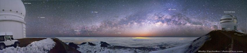
Note:
                                              • UE45a : Matter cycle in the ISM (Charlotte
Syllabus UE 45a                                 Vastel, Katia Ferrière)
                                              • UE45b : Extragalactic physics (Roser Pello)

C. Vastel, 8 lectures
I.   Introduction (First course)
II.  Overview of the ISM (First course)
III. Dust (formation, properties, composition) (Second course)
IV.  Molecular clouds, onset of star formation, shocks from molecular outflows
     (Third course)
V. Neutral gas / HI regions (Third course)
VI. Ionized gas / HII regions (Fourth course)
VII. Photo-dissociation regions (Fourth course)

 K. Ferrière, 2 lectures
       I.     Large-scale shocks and dynamics: supernova remnants and super-bubbles,
              and their impact on the ISM: turbulence, bubbles of hot gas, formation of
              molecular clouds from atomic clouds
       II.    Magnetic field (optical and IR polarization, Zeeman effect, Faraday rotation,
              synchroton emission)
       III.   Cosmic-ray radiation
                                                                                              2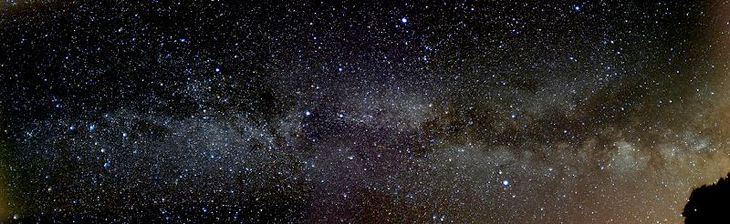
Textbooks, schedule, exam, etc
    ✤   “The Interstellar Medium”, Lequeux
    ✤   "The Physics of the Interstellar Medium", Dyson & Williams
    ✤   “The Physics and Chemistry of the Interstellar Medium”, Tielens
    ✤   “Physical Processes in the Interstellar Medium”, Spitzer
    ✤   “Radiative Processes in Astrophysics”, Rybicki & Lightman
    ✤   http://astro.uwo.ca/~houde/courses/astronomy_9603.html
    ✤   http://www.astronomy.ohio-state.edu/~pogge/Ast871/

✤   Schedule: see http://ezomp2.omp.obs-mip.fr/asep/index.php/Planning

✤   Oral exam in january: present your analysis of a recent article (chosen among
    a given list) and answer course questions.

http://userpages.irap.omp.eu/~cvastel/Welcome_files/M2_2015_2016.html           3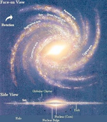
Chapter 1
     Introduction
1.1 A few facts and some definitions
1.2 Historical review of the ISM
1.3 Matter cycle

                                       4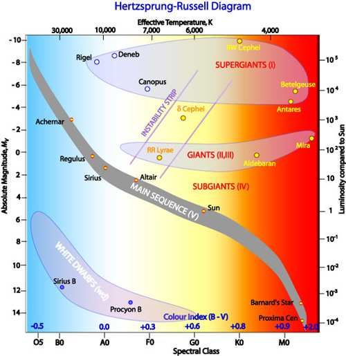
1.1. A few facts and some definitions
Structure of the Universe
Universe                     Galaxy

                                      Ionised        Molecular        Atomic
                                                Interstellar medium            5
                   Stellar systems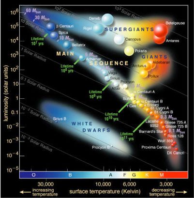
1.1. A few facts and some definitions
    The ISM in the Milky Way (MW)

✤   Molecular gas ~ atomic gas ~ 2×10⁹ M⊙
✤   Total ~ 4×10⁹ M⊙ (1/10 of luminous matter in
    stars)
✤   Assume 2.4×10⁻²⁴ g/H (local abundances)
    ⇒ total number of H nuclei (H, H+, H2) = 3.3×1066
✤   ISM confined to disk of radius ~10 kpc and
    thickness ~200 pc
✤   ⇒ nH ~ 1.8 cm-3
    (Earth’s atmosphere: 2.7×1019 cm-3)                 6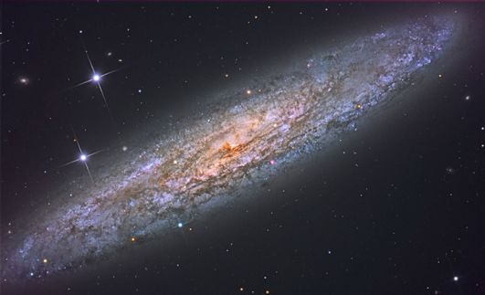
1.1. A few facts and some definitions
Stellar classification
F. 1.1 – Spectres d’étoiles montrant les absorptions dues au gaz autour de l’é
(ex. : celui présent dans l’atmosphère terrestre).
< 1900 >~ 1910
Spectral Atmospheric Hydrogen
Fleming / Spectrum dominated
Secchi Type Temperature (Balmer) Other Features M/M! R/R
Draper by / type of object (K) Features
O > 33, 000 weak Ionized Helium (He+ ) some- 20-60 9-15
I A, B, C, D Hydrogen Balmer times in emission
Strong UV continuum
E, F, G, H, B 10,500-30,000 medium Neutral He absorption 3-18 3.0-8
II Ca, Na
I, K, L A 7,500-10,000 strong H features maximum at A0 2.0-3.0 1.7-2
Some features of heavy ele-
III M Wide bands ments, eg Ca+
F 6,000-7,200 medium 1.1-1.6 1.2-1
IV N Carbon stars G∗ 5,500-6,000 weak Ca+ H&K, Na “D” 0.9-1.05 0.85-1
K 4,000-5,250 v. weak Ca+ , Fe 0.6-0.8 0.65-0
O W-R stars, bright lines Strong molecules, eg CH, CN
M 2,600-3,850 v. weak Molecules, eg TiO 0.08-0.5 0.17-0
P Planetary Nebulae Very red continuum
∗
Sun is G2V
Q Other
Sub-division (0-5) Main sequence H-R diagram
– Les atmosphères des étoiles provoquent des absorptions spécifiques :
(Herzsprung-Russell) 7
Ces absorptions ont été le premier critère de classification des étoiles :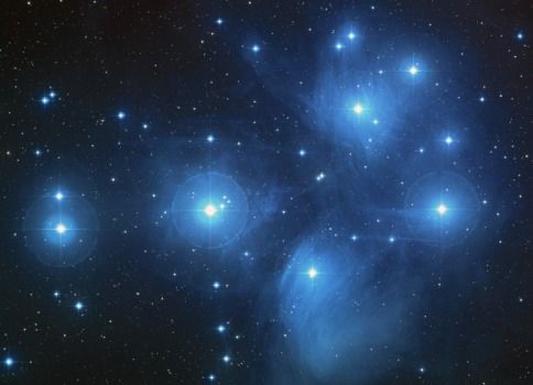
III M Bandes larges
IV N Etoiles carbones
1.1. A few facts and some definitions
O
P
Etoiles Wolf-Rayet, raies brillantes
Nébuleuses planétaires
Stellar classification Q Autres
F. 1.2 – Diagramme de
Hertzsprung-Russell.
Depuis les années 1910, la classification se base sur la température et la luminosité des étoiles (cf.
diagramme H-R) :
Spectral Atmospheric Hydrogen Main
Type Temperature (Balmer) Other Features M/M! R/R! L/L! Sequence
(K) Features Lifetime
O > 33, 000 weak Ionized Helium (He+ ) some- 20-60 9-15 90,000-800,000 10-1 Myr
times in emission
Strong UV continuum
B 10,500-30,000 medium Neutral He absorption 3-18 3.0-8.4 95-52,000 400-11 Myr
A 7,500-10,000 strong H features maximum at A0 2.0-3.0 1.7-2.7 8-55 3 Gyr - 440 Myr
Some features of heavy ele-
ments, eg Ca+
F 6,000-7,200 medium 1.1-1.6 1.2-1.6 2.0-6.5 7-3 Gy
G∗ 5,500-6,000 weak Ca+ H&K, Na “D” 0.9-1.05 0.85-1.1 0.66-1.5 15-8 Gy
K 4,000-5,250 v. weak Ca+ , Fe 0.6-0.8 0.65-0.80 0.10-0.42 17 Gy
Strong molecules, eg CH, CN
M 2,600-3,850 v. weak Molecules, eg TiO 0.08-0.5 0.17-0.63 0.001-0.08 56 Gy
Very red continuum
∗
Sun is G2V
8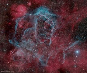
1.1. A few facts and some definitions
    Magnitude, extinction
✤   Hipparchus (-150 av. J-C): apparent magnitude = 1 for the brightest star, 6 for the
    dimmest (to the naked eye)
✤   19th century: eye responds to the difference in
    the logarithms of the brightness ⇒ scale in
    which difference of one magnitude between
    two stars implies constant ratio between their
    brightness

               m = -2.5 log(I/I0)
✤   A difference of 5 magnitudes corresponds
    exactly to a factor 100 in intensity (with the
    smallest magnitude corresponding to the
    highest intensity) :
                      I2
                         = 100(m1 m2 )/5
                      I1                                                                  9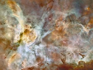
1.1. A few facts and some definitions
      Magnitude, extinction
aille et de la longueur d’onde.
  ✤  Extinction : characterized by extinction coefficient Qext = Qabs + Qsca (absorption
ction+scattering),
      Qext = Qabs +       t.q. : I = I0 exp( ng ⇥a2 Qext ⌥)
                     Qdifthat
                   such

    Measured
 magnitudes
  ✤              as aAmagnitude
             † : soit    le nombredifference:
                                     de magnitudes dû à l’extinction
    let A! the number of magnitudes due to                     I!,0                        I!
ur d’onde entre l’intensité non affectée, I ,0 , et celle observée,
    extinction at a wavelength " between
    I!,0 and I! (observed).
                           I ,0
e, on peut donc écrire :       = 100A /5 = 10A /2.5 , d’où
                            I
  ✤ From the definition of the magnitude, we have :
                                                              I ,0
                            ✓      ◆                                = 100A /5 = 10A /2.5
                           ⇥ I                                 I
    hence A = 2.5I log
     A = 2.5 log              I ,0                                (1.7)
                      I ,0
  ✤ Moreover, we also define the optical depth # such that: I
                                                         !                = I ,0 e ⌧
ion :
      By combining
           I     ⇤
                   the previous equations, we get :
               =e ,                                     (1.8)
          I ,0         A = 2.5 log(e   ⌧
                                          ) = 2.5⌧ ⇥ log e = 1.086⌧
                                                                                                10
1.1. A few facts and some definitions
Distance determination in the ISM
✤ Recall : stellar distances determined by the parallax or by comparison
between apparent and absolute magnitudes (determined from the spectral
type).
✤ Parallax method first used by Friedrich Wilhelm Bessel in 1838 for the
binary star 61 Cyg. D=1AU/tan $ ≈ 1/$ AU
✤ Parsec (pc) = distance for which the annual parallax is 1 arcsec (1/3600 of a
degree) ; e.g. Proxima Centauri has D=1/p(“)=1/0.76=1.32pc
✤ Except for a few cases, method impossible to use for distance
determination of the ISM
✤ For dark (absorbing) clouds, one can use extinction method
111.1. A few facts and some definitions
Distance determination in the ISM
✤ Kinematic distance: determined from the radial velocity of the clouds,
obtained from spectroscopic absorption or emission lines:
✤ galactic disk rotation is not that of a solid body
(same angular velocity, linear velocity ➚ with
radial distance) but it is a differential rotation
(angular velocity ➘ with radial distance) ⇒ all
points along the line of sight have a different
radial velocity.
✤ origin = point close to the Sun, which has a
circular orbit and velocity equal to the mean
velocity of stars in the solar neighborhood
(around 10-20pc)
✤ neighboring stars appear stationary w.r.t Sun
hence the name “Local Standard of Rest” (LSR)
121.1. A few facts and some definitions
Units, abbreviations
✤ “cgs” units (centimeters, grams, seconds) frequently used (instead of
“mks” ⇔ S.I. : meters, kilograms, seconds)
✤ moreover, use of “practical” or “historical” units (e.g., km/s for
velocities, cm-1 for energies) ⇒ take great care with calculations!
✤ Abbreviations for wavelength ranges: NIR (near infra-red), MIR (mid
infra-red), FIR (far infra-red), FUV (far ultra-violet), submm (sub-
millimeter)
10-4nm 1nm 200nm 380nm 780nm 5'm 30'm 200'm 1mm 1cm
"
(-rays X-rays FUV UV VIS NIR MIR FIR cm/
submm mm
radio
& (GHz) 131.2. Historical review of the ISM:
Before the 1900s
✤ Herschel & cie realized that the MW is not just stars in vacuum.
✤ Bright nebulae : “clouds” of gas that do not resolve into stars (when
viewed with a telescope). 3 categories :
diffuse nebulae (e.g.
reflection nebulae) planetary nebulae filamentary nebulae
About planetary nebulae: Herschel
called these spherical clouds planetary
nebulae because they were round like
14
the planets.1.2. Historical review of the ISM:
Before the 1900s
The first reflection nebula, proof of interstellar dust
“...the nebula is disintegrated
matter similar to what we know in
the solar system, in the rings of
Saturn, comets, etc., and...
it shines by reflected star light.”
Slipher, V.M.,Lowell Obs. Bull. 2, 26 (1912)
151.2. Historical review of the ISM:
Before the 1900s
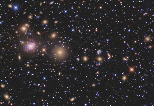
✤ Dark nebulae: originally thought to be holes in the star clouds ; later
recognized to be dark clouds of obscuring material seen in silhouette
against rich star fields.
Especially prominent in the brightest regions of the Milky Way (e.g.,
the Great Rift in Cygnus or the Coal Sack in the Southern Milky Way)
✤ In general, these were viewed as isolated entities in otherwise mostly
empty space, and not as a manifestation of a general ISM.
161
1.2. Historical review of the ISM:
Early 1900s
✤ Johannes Franz Hartmann (January 11, 1865 – September 13, 1936) was a
German physicist and astronomer. In 1904, while studying the spectroscopy of
1904ApJ....19..268H
δ Ori he noticed that most of the spectrum had a shift, which he interpreted as
indicating the presence of interstellar medium.
Black: FUSE observation of LB3459; blue: synthetic stellar spectrum;
red: synthetic stellar spectrum+ISM (Fleig et al. 2008) 171919ApJ....49....
1.2. Historical review of the ISM:
Early 1900s
✤ Barnard (1919): proximity of dark/bright regions
➙ obscuring matter rather than vacuum, blocking
light from more distant stars.
1930PASP...42..214T
✤ Survey of atomic absorption lines convinced astronomers that the space between
stars was filled with interstellar gas, transparent in the visible, except for a few
spectral lines arising from atomic ground states. (but this could not explain the
dark clouds catalogued by Barnard.) Diameter
distance
4000 No absorption
✤ Trumpler effect (1930): apparent diameter of
star cluster ↘ more slowly than their
luminosity ➙ extinction and reddening of
light due to small solid particles (dust Absorption of
grains) mixed with gas. 0.7mag/1000pc
1000
Photometric
distance
1000 4000 181.2. Historical review of the ISM:
Early 1900s
✤ It was Trumpler’s work that produced the most dramatic quantitative proof of
the effect of interstellar matter on the light from stars in clusters. He directly
demonstrated the effect on the apparent diameters of open clusters.
He studied many open cluster and
determined their distance. He
noticed that the apparent diameter
for the more distant clusters
appeared consistently smaller than
expected if they were all the same
typical diameter. In fact, the trend
was so strong that he could not
explain it except to infer that his
original data had been in error. The
brightness of the stars in the more
distant clusters had been dimmed
✤ Trumpler was able to show that the
absorption amounted to about 0.7 by passage through space
magnitudes per kpc. (interstellar matter).
191.2. Historical review of the ISM:
Early 1900s
✤ At the end of the 1930s:
✤ ISM viewed as homogenous and diffuse, pervading space with a nearly
constant density.
High-resolution spectroscopy of stationary lines ➙ complex structure: many
narrower line components with different radial velocities.
⇒ ISM is clumpy and structured into clouds.
✤ Discovery of the 1st molecules : CH (1937), CN (1940)
CH
CN
201.2. Historical review of the ISM:
1940s
✤ Strömgren sphere: Bengt Strömgren ➙ bright diffuse nebulae with strong line
emission = regions of photo-ionized gas surrounding hot stars. These idealized
“Strömgren spheres” are at the heart of our modern theory of ionized nebulae.
✤ 3 types of ionized nebulae: Introduction to the Interstellar Medium
Regions) for the specific objects. Long-established practice and tradition, however, mean that we are
i. H II regions (= “classical” diffuse nebulae ) : characterized by intense line
generally stuck with the confusion. Beware.
At least three basic kinds of ionized nebulae are recognized in the ISM. Note that these are generally
emission ; gas heated and ionized by UV photons
isolated objects, and not to be(h&
discuss later.
confused≥ 13.6eV)
with the ionized phasesfrom
of the generalthe
ISM that we will
atmospheres of embedded O,B stars. H Regions are the classical Fdiffuse nebulae) described by Herschel and others that show strong
II
emission-line spectra. These are regions of interstellar gas heated and ionized by UV (h 13.6eV)
photons from the atmospheres of embedded O and B stars.
Nomenclature : spectroscopically, H II refers to ionized hydrogen
(H+), which can be present in a number of unrelated objets. The
term “H II regions” specifically refers to the bright diffuse
nebulae described here. H+ is not confined to discrete regions, but
is observed in the entire ISM; in fact, ~ 90% of H+ in the MW is
outside classical H II regions : it is the WIM (warm ionized
medium). (So it is not because there is some H+ that it is an H II
region.) 211.2. Historical review of the ISM:
1940s
✤ 3 types of ionized nebulae (ctd):
ii. planetary nebulae (PN) : UV photo-ionized
ejected stellar envelopes surrounding hot
remnant stellar core (white dwarf)
‣ Note : H II regions and PN = similar
manifestation of 2 different processes
(stellar birth vs stellar death)
iii. SuperNova Remnants (SNRs): regions ionized by the passage of a blast
wave from SN explosion; differ from the previous 2 by the source of ionizing
photons and the additional heating mechanism.
22Supernova Remnants (SNRs). These are regions ionized by the passage of a blast
supernova explosion through the ISM (either Type I or Type II supernovae). They d
1.2. Historical review of the ISM:
regions and PNe in the source of ionizing photons and the additional mechanical hea
hydrodynamical shockwave. Two basic types of SNRs are recognized:
Young SNRs (e.g., Crab Nebula) are photoionized by UV synchrotron radiation emi
relativistic electrons accelerated by the central pulsar. These are often called JPlerion
Introduction
crab-like)toafter
the Interstellar
the prototypeMedium
Crab Nebula in Taurus (remnant of SN1054).
1940s Supernova Remnants (SNRs). These are regions ionized by the passage of a blas
supernova explosion through the ISM (either Type I or Type II supernovae). They
regions and PNe in the source of ionizing photons and the additional mechanical he
hydrodynamical shockwave. Two basic types of SNRs are recognized:
Young SNRs (e.g., Crab Nebula) are photoionized by UV synchrotron radiation em
relativistic electrons accelerated by the central pulsar. These are often called JPlerio
crab-like) after the prototype Crab Nebula in Taurus (remnant of SN1054).
✤ 3 types of ionized nebulae (SNRs, ctd):
✤ young SNRs (e.g. Crab Nebula) : photo-ionized Figure I-4: Crab Nebula, young SNR (AD1054). [Credit: VLT Kueyen+FORS2
by synchrotron radiation emitted by relativistic e− Old SNRs (e.g., Cygnus Loop), which are photoionized by X-rays emitted from den
regions collisionally heated to 105 6K by the passage of the supernova blast wave thr
accelerated by the central pulsar ISM. Most of the gas in the remnants has been plowed up by the shock, and we see t
where the gas has reached temperatures of ~104 K (where line emission is most effic
see later).
✤ old SNRs (e.g., Cygnus Loop) : photo-ionized by Figure I-4: Crab Nebula, young SNR (AD1054). [Credit: VLT Kueyen+FORS
X-rays emitted by cooling of dense regions heated Old SNRs (e.g., Cygnus Loop), which are photoionized by X-rays emitted from de
5 6
regions collisionally heated to 10 K by the passage of the supernova blast wave th
to 105−6 K by collisions due to the passage of a shock
ISM. Most of the gas in the remnants has been plowed up by the shock, and we see
where the gas has reached temperatures of ~10 K (where line emission is most effi 4
see later).
wave from the SN in the ambient ISM.
Figure I-5: The Cygnus Loop, an old SNR. This image shows emission from the
shockwaves impinging on the ambient ISM (sharp filaments). [Credit/Copyright:
Jerry Lodriguss, www.astropix.com]
✤ Strömgren’s work led to the recognition that the spectra of photo-ionized regions I-5
contained a number of important diagnostics of the physical state of the gas
(density, temperature, abundances, etc), which is now a major research field.
Figure I-5: The Cygnus Loop, an old SNR. This image shows emission from the
shockwaves impinging on the ambient ISM (sharp filaments). [Credit/Copyright:
Jerry Lodriguss, www.astropix.com]
I-5
231.2. Historical review of the ISM:
1950s-1970s
✤ Line emission from cold (10K) neutral hydrogen
atoms at 21-cm via hyperfine atomic transitions in
the ground state predicted in 1945 by van de Hulst,
and first detected in 1951 by Ewen and Purcell at
Harvard (followed 6 weeks later by the Dutch
astronomers Muller and Oort)
Cold H I clouds = majority of the total mass of the ISM.
✤ This discovery initiated the era of radio-wavelength studies of the ISM, and was
the beginning of using the ISM to trace out Galactic structure.
✤ cm: OH @ 18cm (Weinreb et al. 1963), NH3 @ 1.25cm (Cheung et al. 1968),
H2O @ 1 cm (22 GHz) (Cheung et al. 1969)
✤ mm: CO @ 2.7 mm (Wilson, Jefferts & Penzias 1970)
✤ UV (space): H2 in 1970
✤ >130 molecules detected: http://www.astro.uni-koeln.de/cdms/molecules
241.3. Matter cycle
251.3. Matter cycle
Diffuse
26Example for warming-up...
On donne la luminance L d’une étoile de rayon R. On souhaite calculer la puissance
totale reçue par une planète de rayon Rp et tournant à distance d de son étoile.
Data:
L = 107 W/m2/sr d = 1.496 108 km
R = 6.96 108 m Sd = 2 cm2
Rp = 6378 km t = 1 minute
1) Quelle surface A de l’étoile est visible à chaque instant depuis un objet
orbitant autour d’elle?
2) Calculer l’angle solide Ω sous lequel est vu la planète depuis n’importe quel
point de la surface de l’étoile.
NB: Pour calculer l'angle solide sous lequel on voit un
objet à partir d'un point donné, on projete l'objet sur
une sphère de rayon R centrée en ce point. L'espace
complet est vu sous un angle solide de 4π stéradians.
Ω = A/r2
27Example for warming-up...
1) Quelle surface A de l’étoile est visible à chaque instant depuis un objet
orbitant autour d’elle?
La surface totale de l’étoile est 4πR2. Seule la
moitié de l’étoile est visible à chaque instant,
donc A= 2πR2.
L’objet orbitant autour de l’étoile est evidemment sufisemment loin pour être considéré
comme un point.
AN: A=3.04 1018 m2
282) Calculer l’angle solide Ω sous lequel est vu la planète depuis n’importe quel point
de la surface de l’étoile.
L’objet orbitant autour de l’étoile est evidemment sufisemment loin pour être
considéré comme un point: disque non courbé.
Par définition d’un angle solide, Ω=π Rp2/d2, car la planète est vue comme un disque
depuis l’étoile,
AN : Ω=5.77 10-9 sr
Pour calculer l'angle solide sous lequel on voit un objet à partir d'un point donné, on projete
l'objet sur une sphère de rayon R centrée en ce point. L'espace complet est vu sous un angle
solide de 4! sr.
29Example for warming-up...
Données:
L = 107 W/m2/sr
R = 6.96 108 m
Rp = 6378 km
d = 1.496 108 km
Sd = 2 cm2
t = 1 minute
3) Calculer le flux Φ (en Watts) émis par la surface A de l’étoile dans l’angle
solide Ω. Φ représente la puissance lumineuse totale reçue par la planète.
4) Calculer l’éclairement moyen E (en W/m2) reçu sur la planète, hors atmosphère
(considérer dans ce cas la planète comme un disque)..
5) En déduire le flux Φd reçu par le détecteur et l’énergie Qd (en Joules)
absorbée pendant le temps t.
303) Calculer le flux Φ (en Watts) émis par la surface A de l’étoile dans l’angle
solide Ω. Φ représente la puissance lumineuse totale reçue par la planète.
Analyse dimensionnelle!!! La luminance L donne le flux par unité d’aire et par unité
d’angle solide. Donc Φ=LxAxΩ
AN: Φ=1.75 1017 W
4) Calculer l’éclairement E (en W/m2) moyen reçu sur la planète, hors atmosphère
(considérer dans ce cas la planète comme un disque).
A la verticale de l’étoile, l’éclairement reçu sur la planète est E=Φ/π Rp2
E=LxAxΩ/π Rp2 = 107x 2πR2x(π Rp2/d2)/π Rp2
AN: E= 107x 2πR2/d2=1367 W/m2.
5) En déduire le flux Φd reçu par le détecteur et l’énergie Qd (en Joules)
absorbée pendant le temps t.
Le flux reçu par le détecteur vaut Φd =ExSd et il correspond à une énergie Qd=Φd xt
AN: Φd=0.27 W et Qd=16.2 J.
31You can also read