Medium Frequency Range Analysis in non-homogeneous slender structures
←
→
Page content transcription
If your browser does not render page correctly, please read the page content below
21ème Congrès Français de Mécanique                                   Bordeaux, 26 au 30 août 2013

Medium Frequency Range Analysis in non-homogeneous
                slender structures
                                          P. Giberta , E. Gaya
              a. MEcanique et DYnamique des SYStemes 8bis bd Dubreuil 91400 Orsay

Résumé :
Des phénomènes de propagation d’ondes dans des milieux homogènes ou non interviennent dans de
nombreux domaines de la physique. En mécanique on utilise notamment le principe des ondes guidées
lors de l’inspection de panneaux composites par Contrôle Non Destructif. Nous proposons une méthode
numérique simplifiée permettant de déterminer les chemins de propagation d’ondes dans des struc-
tures élancées, non homogènes, dans le cas où la longueur d’onde est de l’ordre de grandeur de la
dimension transverse, et petite par rapport à une dimension longitudinale macroscopique du système.
Pour cela on utilise une méthode asymptotique de type W.K.B.J., dont la résolution à l’ordre un se
ramène à un système Hamiltonien construit à partir des propriétés propagatives locales et dont les
trajectoires fournissent les chemins de propagation. Les lois de conservation de l’énergie obtenues à
l’ordre deux permettent de déduire la localisation des zones de concentration d’énergie engendrées par
l’hétérogénéité.

Abstract :
A lot of physics fields involve wave propagation within non-homogeneous materials. Numerous methods
use guided waves in slender bodies such as composite laminates to verify their integrity, especially for
the Non Destructive Inspection of aircraft structures, or to identify their mechanical properties. A
simplified numerical approach of the wave propagation within non-homogeneous slender structures is
proposed here. In our conditions, the wavelength is significantly smaller than the characteristic ma-
croscopic length of the structure but it is in the same range as the transverse size. The Finite Element
approach is impossible in this case. A specific asymptotic approach based on W.K.B.J. method is then
used. A first-order non linear partial derivative equation is set up using the material local propagative
properties and is solved using an Hamiltonian system. The energy propagation is thus precisely descri-
bed. The propagation of energy could be deviated depending on the material heterogeneities and some
areas are submitted to energy concentration.

Mots clefs :      guided waves ; non-homogeneous slender structures ; composite materials

1    Introduction
Numerous physical fields involve waves propagation, either in three-dimensional material, or in one
or two-dimensional waves-guides. The detection and identification of defects and damaged areas are
provided through the measurements of the propagative properties of guided waves [1, 4]. Numerous
papers deal with theoretical or experimental applications, in civil engineering - inspection of aging civil
structures, for example after earthquakes, aircraft engineering - Non Destructive Testing of composite
components. These studies concern a special kind of guided wave : the Lamb waves. The detection of
various kinds of defect has been investigated : porosity, moisture, thermic deterioration or delamination
of composite material can be detected using this method.
The finite elements approach of the high frequency analysis raises the question of compatibility bet-
ween the mesh size and the wavelength or material heterogeneity. For complex materials such as

                                                    1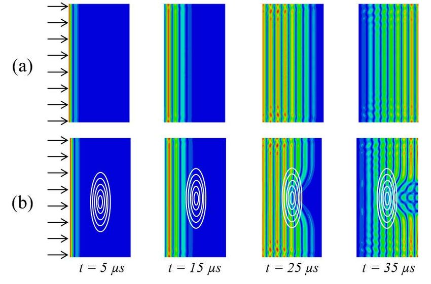
21ème Congrès Français de Mécanique                                                            Bordeaux, 26 au 30 août 2013

composites laminates with a periodic microstructure, the phenomena at different scales could interfere
with each other. The global vibrational behavior depends on the wavelength and several frequency
ranges may coexist as well as several models of vibrational behaviors. In some complex cases, it is even
possible to observe three scales : the macroscopic dimension or thickness of a plate, the period of the
representative elementary model, and the wavelength. A comparison between these scales is required
to define simplified models. On the other hand, the numerical determination of the propagative pro-
perties of waveguide with constant longitudinal properties have already been reported, for example
for the propagation of Lamb waves in multi-layered composites [2].
The wave propagation is here studied within non-homogeneous materials with a distributed hete-
rogeneity. This heterogeneity could have been induced by a mechanical deformation, it could be a
distributed defect generated during the manufacturing process or in use. This defect is either physical
(for example a variation of the thickness or a local curvature of the a plate) or mechanical (non-
constant constitutive behaviour law). This paper aims to demonstrate that it is possible to completely
predict the propagation of energy, the local energy concentration and the extinction of modes along
virtual boundaries, using a simplified numerical approach. This analysis and related numerical tools
could support experimentation to detect and identify the distributed defects.
The well-known W.K.B.J. asymptotic method is used and adjusted by introducing a small scale
parameter that determines the wavelength depending on a macroscopic characteristic length. The wa-
velength is supposed to have a similar size than the transverse dimension of the waveguides. After the
description of the mechanical process of the method in section 2, the first and second order approxi-
mations are studied in sections 3 and 4. In section 5, the method is illustrated using examples and the
multi-purpose MFRA.Waves software is introduced.

2    The mechanical context - The W.K.B.J. method
The shell is defined as a tridimensional structure using its mid-surface Γ and its constant thickness
h = L , where  is a scale parameter considered small and L is the given reference macroscopic length.
D is the physical domain defined by the relation (1) :

                                                                  h      h

                                          m(τ1 , τ2 )
                             D = {M =                   , m ∈ Γ, − < z < }                           (1)
                                              z                   2        2

where τ1 , τ2 are the curvilinear coordinates of m on Γ and D is the stretched and fixed domain :

                                        m(τ1 , τ2 )             L     L
                                D={                   , m ∈ Γ, − < Z < }                          (2)
                                           Z                    2     2

The unitary tangent vectors a,α are defined so that m,α = Aα .a,α , α = 1, 2 and aα , α = 1, 2 are
supposed orthogonal as a simplifying assumption.
The elastic waves propagate along the mid-surface Γ with a wavelength in the same range as the
shell thickness. The frequencies are thus given as a function of 1 . As a consequence, the terminology
Medium Frequency Range is used.
The W.K.B.J. method [3, 7] is used to evaluate the propagative tridimensional solutions. Then for a
pulsation ω  = Ω at a given Ω, tridimensional solutions are considered as :
                                                               S(τ1 ,τ2 )                         z
                            u(τ1 , τ2 , z, t) = eiω       t−i               .U  (τ1 , τ2 , Z =     )                       (3)


U  is then gradually determined using the asymptotic expansion :

                                      U  = U0 +  U1 + 2 U2 + . . .                                                        (4)

Then the new unknown parameters are the phase S(τ1 , τ2 ), and the induced displacements U0 (τ1 , τ2 ),
U1 (τ1 , τ2 ), etc

                                                                2
21ème Congrès Français de Mécanique Bordeaux, 26 au 30 août 2013
The solution is locally related to a waveguide mode for an infinite plate :
−kloc1 Xloc1 −kloc2 Xloc2 )
u ≈ C cst ei(Ωt U0 (0, 0, Z) (5)
1
where klocα = Aα (0,0) S,α (0, 0), α = 1, 2 with S,α = τ∂S
∂α
and C cst is a constant, Xlocj , j = 1, 2 are the
local cartesian coordinates and t = t the fast time.
(5) is a waveguide solution relation for the tangent infinite plate at (0, 0), where the mechanical
properties are the same as those at (0, 0). The general solution (3) is thus locally a waveguide eigenmode
at frequency Ω and S is closely related to the local wave number and then to the wavelength.
S, U0 , U1 are now determined step by step using the asymptotic expansions method in a global
variational formulation of a dynamical problem, on tridimensional space of variables τ1 , τ2 , Z.
The strain (6,1) vector is then derived for a displacement u using relation (3) as a function of the
amplitude U in the local coordinate system (time t is not taken into account) :
1
(u) = {−iLS 0 (U ) + g (U )} + {m (U ) + A.U − iZMS 0 (U )} + {...} (6)
with :
LS 0 (U )tr = S10 U1 S20 U2 0 S20 UZ S10 UZ S10 U2 + S20 U1
(7)
tr ∂UZ ∂U2 ∂U1
g (U ) = 0 0 ∂Z ∂Z ∂Z 0 (8)
m (U )tr = 1 ∂U1
A1 ∂τ1
1 ∂U2
A2 ∂τ2 0 1 ∂UZ
A2 ∂τ2
1 ∂UZ
A1 ∂τ1
1 ∂U2
A1 ∂τ1 + 1 ∂U1
A2 ∂τ2 (9)
MS 0 (U )tr = S10 R
U1
S20 R
U2
0 S20 URZ2 S10 URZ1 S10 R
U2
+ S20 R
U1
1 2 1 2
(10)
and A is a (6,3) matrix that only depends on the local geometry of the mid-surface Γ.
S(τ1 ,τ2 )
A virtual displacement is chosen with a similar relation : v(τ1 , τ2 , z, t) = eiω t−i .V (τ1 , τ2 , Z = z )
with compact support in D, the dynamical equations are derived using a variational formulation given
by : R
1 tr
D { (−iLS 0 (U ) + g (U )) + (m (U ) + A.U − iZMS 0 (U )) + ...} .C.
1 ∗ ∗ ∗ ∗ ∗
{ (iLS 0 (V ) + g (V )) + (m (V ) + A.V + iZMS 0 (V )) + ...}dD = (11)
Ω2 tr ∗ 3
R
= 2 D ρU .V dD ∀V : D → <
where dD = A1 A2 dτ1 dτ2 dZ, and V has a compact support in21ème Congrès Français de Mécanique Bordeaux, 26 au 30 août 2013
3 The eikonale equation
In the relation (12) the point (τ1 , τ2 ) is considered as a parameter ; it can be rewritten as the variational
equation along the thickness of a waveguide problem given at the point (τ1 , τ2 ) and using its mechanical
characteristics :
Z L Z L
2 2
(g (U 0 ) − i.Lk (U 0 ))tr .C(τ1 , τ2 , Z).(g (V ∗ ) + i.Lk (V ∗ )) dZ = Ω2 ρ(τ1 , τ2 ) U tr ∗
0 .V dZ
−L
2
−L
2
L L L L
U 0 (τ1 , τ2 , .) : ] − , [→21ème Congrès Français de Mécanique Bordeaux, 26 au 30 août 2013
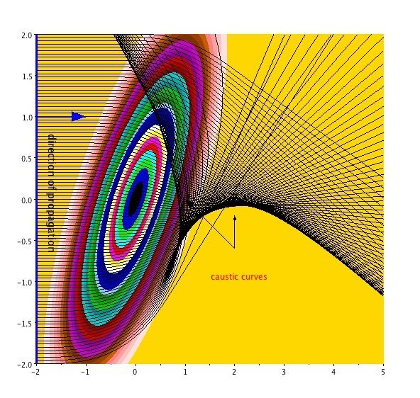
close to the caustic curves (envelopes of the trajectories, see Figure 1). As explained in the next
section, these areas are submitted to a concentration of energy and asymptotic expansion (4). The use
of the exponential function is not relevant anymore because the kind of solution has changed. A local
analysis has to be carried, using specific Airy functions and a multiple scale asymptotic expansion [3].
The trajectories and then the energy are deviated and attracted near the singular points χ0 for equation
(22) such that ψ(χ0 ) = ψ 0 (χ0 ) = 0. For example, a point with a minimal cut-off frequency is singular.
As the adequate eigenmode is chosen depending on the kind of damage, such points are linked to the
maximal damage. Other phenomena may occur for eigenmodes with a null group velocity [6].
Figure 1 – Wave propagation within a composite plate with a degradation of the behaviour law. A
caustic curve is generated after this damaged area.
4 The transport equation
The equation (13) can be considered as a forced response equation for an unknown displacement U1
induced by a loading depending on φ. The Fredholm condition shows the existence of a solution and
a new equation is obtained to determine φ, and then the first order solution U0 is completed. If only
the modulus of φ is taken into account, depending on the local energy of the wave, this equation can
be given by :
∂H 0
div(|φ|2 (S , x)) = 0 (23)
∂k
Then the square of the wave amplitude times the group velocity of the wave is constant along a
trajectory. The wave paths are directly linked to the way energy propagates. As explained earlier,
some complex situations may occur, leading to a concentration of energy. This phenomena could be
localized after a defect where the wave is refracted, or ahead the boundaries of a forbidden frequency
zone.
5 Software development
The authors have developed the MFRA.Waves software (Medium Frequency Range Analysis) to sup-
port experimental Non Destructive Inspection. It has the ability to calculate waves propagative pro-
perties within multi-layered materials. It also takes into account the interaction of the waves with
continuous damage in structures such as beam, plate and shell. Medium Frequency Range waves are
considered as a particles flow whose trajectory is related to energy concentration as described in this
paper. Figure 2 provides a comparison of wave propagation within an intact plate and a damaged one.
521ème Congrès Français de Mécanique Bordeaux, 26 au 30 août 2013
The damage is modeled as a continuous decrease of the Young’s modulus, represented in the figure by
the white ellipses.
Figure 2 – Wave propagation within a composite plate :(a) Intact, and (b) With a continuous damage.
Parameters used to model the plate and solicitation are : plate dimension : 3 ∗ 150 ∗ 75 mm, density
= 1.53, EL = 20 GPa, ET = 8 GPa, GLT = 4 GPa, frequency = 233 kHz, mode S0
Wave propagation is altered by this degradation. The software MFRA.Waves provides thus a valuable
support to interpret the experimental response of the laminate to a wave solicitation.
6 Conclusion
The method provides a numerical solution for medium frequency wave propagation in composite slen-
der structure. It is based on a semi-analytical approximation using a W.K.B.J. asymptotic expansion.
It uses the local propagation properties, such as the relations of dispersion, to solve a first-order nonli-
near partial derivative equation using a characteristic method. The wave propagation is then described
by the particles movements computed by a Hamilton equation solver. The local displacements and the
wave vectors as well as the magnitude of the energy are determined using this method. The energy
concentration areas are highlighted through the post-processing of the trajectories after solving the
Hamilton equations. An heterogeneity induces a perturbation of the distribution of energy : some areas
are submitted to a concentration of energy while other ones receive less energy.
Future works will concern the application of the method to other fields of physics such as electroma-
gnetism or optics.
Références
[1] Y. Bar-Cohen, A. Mai, Z. Chang 1998 Defects detection and Characterization using Leaky Lamb
wave (LLW) dispersion data, Proceeding of the ASNT Asia-Pacific Conference on NDT. and 7th
Annual Research Symposium, Anaheim, CA, 24-26 March.
[2] M. El Allami, H. Rhimini, M. Sidki 2010 Propagation des ondes de Lamb : Résolution par la
methode des éléments finis et post-traitement par la transformée en ondelettes, Compte-rendu du
10eme Congres Francais d’Acoustique, Lyon, 12-16 avril 2010.
[3] Ali Nayfeh Perturbation methods, Pure and Applied Mathematics - Wiley-Interscience Publications
(1973)
[4] A. Raghavan, C.E.S. Cesnik 2007 Review of guided-wave structural health monitoring, The Shock
and Vibration Digest, 39 no 2, 91-114
[5] D. Royer, E. Dieulesaint, Ondes elastiques dans les solides, Tome 1 : Propagation libre et guidée
Ed. Masson (1996)
[6] D. Royer, D. Clorennec, C. Prada 2010 Caracterisation de plaques et de tubes par modes de Lamb
a vitesse de groupe nulle, I2M - 10/2010 Méthodes innovantes en CND 73-94
[7] M.A.Slawinski Waves and Rays in Elastic Continua World Scientific Publishing Co.Pte.Ltd. (2007)
6You can also read