Cellular digitized map on Google Earth - Galib Hashmi1, Saleh Faruque1
←
→
Page content transcription
If your browser does not render page correctly, please read the page content below
IOSR Journal of Electronics and Communication Engineering (IOSR-JECE)
e-ISSN: 2278-2834,p- ISSN: 2278-8735. Volume 7, Issue 5 (Sep. - Oct. 2013), PP 13-17
www.iosrjournals.org

                        Cellular digitized map on Google Earth
                                   Galib Hashmi1, Saleh Faruque1
 1
     (Department of Applied Physics, Electronics & Communication Engineering, Dhaka University, Bangladesh)

 Abstract: While designing a cellular network, the main issue for the network planning is to achieve maximum
capacity while maintaining an acceptable grade of service and good speech quality. Planning an immature
network does not allow future growth and expansion. Wise & calculative re-use of site location in the future
network structure will save money for the operator. For this reason, digital maps are one of the most essential
elements to the network engineers while they have to think about expanding their business. However, the digital
maps cost a lot of money. This problem can be mitigated if Google Earth is used.
         In this paper, the procedure of how to design a cellular digitized map on Google Earth is shown. By
calculating the cell radius, implementing the single cell site, forming the 7-cell cluster and all the cells a low
cost digitized map is designed. It is necessary to have a digitized map in mobile communication because
ultimate goal includes efficient usage of RF wave, frequency reuse, total use of BW and last but not the least
cost reduction.
Keywords: Cellular digitized map, Cell radius, Google Earth.

                                         I.          INTRODUCTION
          The Mobile communication is currently at its fastest growth period in history; due to enabling
technologies, which permit wide spread deployment. The early land to mobile radio systems used a single high-
powered transmitter with an antenna mounted on a tall tower to achieve a large coverage area. There was
generally no in system interference as the same frequencies were reused in the next service area which used to
be several hundred miles away. But because of the rapid growth and need for high quality and high capacity
cellular networks in recent years, single high-powered transmitter with single frequency are not used. Scientists
combined the cells into groups called cluster, where no frequencies are reused within a cluster. Frequencies used
in one cell cluster can be reused in another cluster of cells. A large number of cells per cluster arrangement
reduces interference to the system, and increases the system’s capacity and efficiency. In today’s world
normally a 7- cell cluster is used in a mobile communication system. Figure 1 shows earlier single cell & todays
cluster cell format.
          Once cell cluster is formed, RF propagation of each mobile phone cell tower is needs to be known. For
that estimating coverage accurately has become extremely important to provide high quality and high capacity.
From generic RF propagation prediction algorithms based on computer databases or empirical results give only
approximate coverage, but do not show the coverage area on the map. In addition to design, more accurately the
coverage of modern cellular networks, signal strength measurements must be taken in the service area using a
test transmitter. Taking signal strength measurements is an expensive and time consuming task so the exact cell
radius is to be known. Otherwise, there will be excessive drive testing, and the true accuracy of RF coverage
will not be predicted. So before drive testing we have to know the cell radius that is the cell radius must be
mapped. Various companies are providing digitized map, where the cell radius can be drawn before cell tower
implementation and drive test.
          However, this digitized map, provided by the various companies, cost a fortune and thus implementing
a cell tower is expensive. Therefore, to reduce cost, cellular digitized map forming a 7- cell cluster or a map
showing all the clusters can be designed on Google earth. Here in this paper at first a cell radius is drawn
(Okumura- Hata is used as a prediction model to calculate the cell radius), and then 7- cell cluster is drawn on
the Google Earth and thus making of a digitized map.

       Fig.1 Illustration showing the early mobile communication single cell & todays cluster cell format
                                              www.iosrjournals.org                                      13 | Page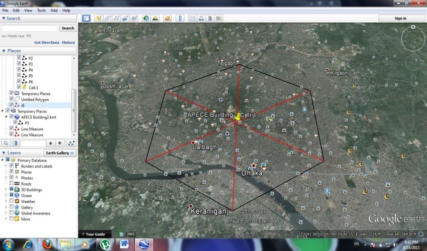
Cellular digitized map on Google Earth
II. COVERAGE ESTIMATION TECHNIQUES: EMPIRICAL MODELS
The For the mobile communication systems, the coverage estimation is mostly based on simple
empirical propagation models. The empirical models are developed for different morphologies for some typical
cities, and are limited to the ability of the engineers to classify the morphology and only provide an approximate
estimate of coverage. In case of first generation mobile phone systems only one base station was used, and
prediction was used to determine the approximate boundary where the subscribers could use the service.
The situation in modern cellular systems is different. The modern cellular systems are being built to provide
high quality of service (QOS) and high capacity. To minimize the interference (adjacent and co-channel channel
interference) it is important to determine the coverage boundary accurately. Predicting inaccurate coverage has
severe impact on the network performance. Overestimating coverage will result, areas with signal strengths
weaker than the minimum required threshold. Underestimating coverage will create interference because of
coverage overlap. Thus, accurate estimation of coverage is essential for a good design.
Among numerous propagation models, the following are the most significant ones, providing the founding of
today’s land- mobile communication services:
1) The Okumura- Hata model
2) The Walfisch Ikegami model
Here in this project Hata urban model is being used. Details about Hata model is described in the next section.
III. PROPAGATION PATH LOSS
A very important measure of interest in radio propagation is the path loss, which is defined as the ratio
between the received power Pr and the transmitted power Pt,
Ld = Pr/Pt
Propagation models are used to determine cell sites are required to provide the coverage requirement for the
networks. Initial network design typically is engineered for coverage. Later network growth is based on
capacity. The propagation model helps to determine where the cell sites should be located to achieve an optimal
position in the network. If the propagation model used is not effective in placing cell sites correctly, the
probability of incorrectly deploying cell sites into the network is high. The propagation model is also used in
other system performance aspects including handover optimization, power level adjustments and antenna
placements. Predictions of signal strength and propagation coverage area are vital aspects in the design of
wireless communication systems. There are several methods for finding the propagation loss as follows:
Hata-Okumura
Walfisch-Ikegami
Lee model
The number of Epstien-Peterson
Phenomena like multipath propagation, reflection, diffraction and shadowing have a significant influence on the
received power. Therefore, the propagation models should consider these phenomena to obtain precise results.
In the present study, HATA model is considered for Dhaka city, Bangladesh. Dhaka city being a megacity,
adjusts well with HATA model which is suitable for urban or dense urban area.
IV. HATA-OKUMURA PROPAGATION MODEL
Among the many important technical reports that are concerned with propagation prediction methods
for mobile radio, Okumura’s report is believed to be the most comprehensive one for urban and dense urban
area. In his paper, many useful curves were used to predict the median value of the received signal strength is
presented based on the data collected in the Tokyo area. The Tokyo urban area was then used as a basic
predictor for urban areas [So the Hata- Okumura model is used for Dhaka city]. The correction factors for
suburban and open areas are determined based on the transmit frequency. Based on Okumura’s prediction
curves, empirical formula for the median path loss, Lp, between two isotropic antennas, were obtained by Hata
and are known as the Hata Empirical Formula for Path Loss. The Hata propagation formulae are used with the
link budget calculation to translate a path loss value to a forward link cell radius and a reverse link cell radius.
The Hata model illustrate a slightly more complicated path loss model that is a function of parameters such as
frequency, frequency range, heights of transmitter and receiver, and building density. The Hata model is based
on extensive empirical measurements taken in urban environments. In its decibel form, the generalized model
can be written as –
LP = C1 + C2 log (fmhz) – 13.82 log (hb) – a(hm) + [44.9 – 6.55 log (hb)] log (dkm) + C0
Where,
Lp is the path loss,
www.iosrjournals.org 14 | Page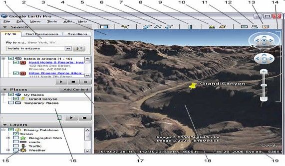
Cellular digitized map on Google Earth

f is the carrier frequency (in megahertz),
h is the antenna height (in meters) of the base station,
 b
h is the mobile antenna height (in meters),
 m
d is the distance (in kilometers) between the base station and the mobile user.
For these parameters, there are only certain ranges in which the model is valid; here we have considered h as
                                                                                                                                  b
30m. h as 2m, and d should be between 1 km to 20 km.
         m
In this project d is 3.4 km, which can be calculated from path loss and vice versa. The equation of the slope is γ
= [44.9 – 6.55 log (hb)]/ 10
The terms a(h ) and C are used to account for whether the propagation takes place in an “urban” or a “dense
                m           o
urban” environment. In particular,
a(h ) = [1.1 log (f) – 0.7] h – [1.56 log (f) – 0.8] for “urban” or
     m                             m
                                  2
a(h ) = 3.2[log (11.75h )] – 4.97 for “dense urban”
     m                      m
And
C =0 for “urban”, or
 0
C =3dB for “dense urban”
 0
The term C1 and the factor C2 are used to account for the frequency ranges. Specifically,
C =69.55 for frequency range 150 ≤ f ≤ 1000 MHz, or
 1
C =46.3 for frequency range 1500 ≤ f ≥ 2000 MHz
 1
And
C =26.16 for frequency range 150 ≤ f ≤ 1000 MHz, or
 2
C =33.9 for frequency range 1500 ≤ f ≥ 2000 MHz
 2
According to Hata model the path loss is expressed as,
LP=69.55+26.16log (f)-13.82log h -(1.1 log f-0.7) h + (1.56 log (f)-0.8) + (44.9-6.55log h ) log (d)
                                          b                    m                                            b
From the above equation, the Path loss and Cell radius can be calculated. The calculation is solved in Microsoft
Excel, and the calculation is showed in table I.

                                                 V.            CALCULATION
                                  Table I. Path loss (Lp) and cell radius (d) calculation
         Frequency   C0         C1      C2                  a(hm)         Gr                                Rsl        Rsl
                                                Hb    Hm                         ERP    d(km)    Lp
         (Mhz)       (dB)       (dB)    (dB)                 urban        (dB)                              (db)       (dBm)
                                                                                                                 -           -
              900      0        69.55   26.26   30     2     1.29071        3    22.1     3.38   143.7595
                                                                                                            118.75     88.7495
                                                                                                                 -           -
             1500      3         46.3    33.9   30     2     1.43269        3    22.1       3    151.9295
                                                                                                            126.92     96.9195
                                                                                                                 -           -
             1200      3         46.3    33.9   40    1.5   0.027126        3    22.1      3.5   150.2361
                                                                                                            125.23     95.2261
                                                                                                                 -           -
              800      0        69.55   26.26   40    1.5   0.011278        3    22.1      3.4   141.6294
                                                                                                            116.62     86.6194
                                                                                                                             -
             1000      0        69.55   26.26   30     2           1.32     3    22.1   3.3978   145.0076       -120
                                                                                                                       89.9976

From the above table, the cell radius can be calculated, and cell radius can be easily drawn on the Google Earth.
However before drawing, knowledge about Google Earth is necessary.

                                                VI.           GOOGLE EARTH
          Google Earth is a program that allows the user to view the Earth from space. Once an address is typed
in, the user is “transported” there to view 3D terrain and buildings. The user is in the driver’s seat, controlling
the zoom, tilt and directionality. It is a free program that has an endless number of home, school and business
uses.
Google earth contains:
     • Overhead Satellite and Aerial Imagery
     • Highway Maps
     • Ability to create and save Placemarks and folders
     • Integration with Internet resources
     • 3D Landforms and 3D Buildings

                                                      www.iosrjournals.org                                                   15 | Page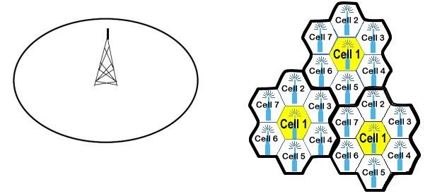
Cellular digitized map on Google Earth
• Network Connections for real-time data monitoring
• Tools for measuring and creating paths
• Ability to create image overlays
Fig.2 Google earth main window
VII. CELLULAR DIGITIZED MAP
By using the data from table I, and using the measure tool in Goggle Earth, the cell radius can be
drawn, on the Google earth. The RF cell coverage on Google Earth is shown in the following figure 3.
Fig.3 Google Earth showing single cell cellular RF coverage
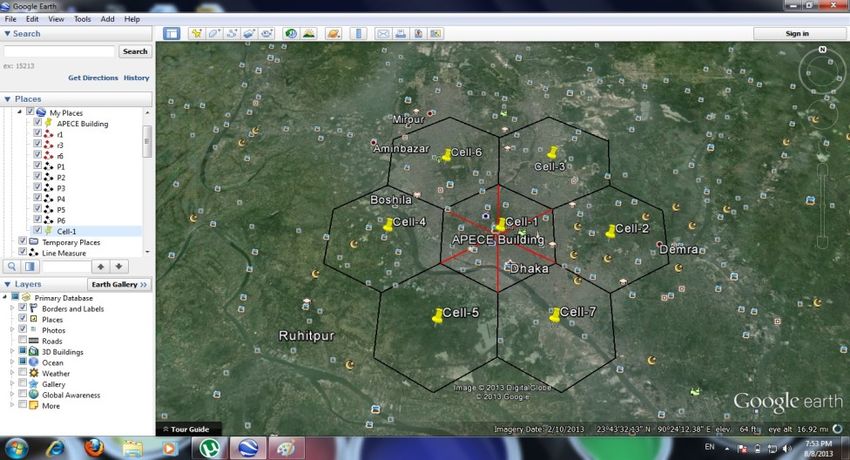
If cell drawing is continued by using the measurement tool in Google Earth, a 7-cell cluster is formed on Google
Earth, shown in figure 4. Also by clicking the cell number in places panel on the left side of Google Earth on
can select any cell, and travel very quickly to the required cell coverage area. Every cell is represented by a
yellow pin and a cell number. According to the user need cell clusters can be drawn and these cell clusters can
cover whole nation or city and thus making of a fully developed digitized map on Google Earth.
Fig.4 Google Earth showing 7- cell cluster
www.iosrjournals.org 16 | PageCellular digitized map on Google Earth
VIII. CONCLUSION
This paper presents an innovative approach of designing cellular digitized map on Google earth.
Accurate modeling of cellular RF coverage is of vital importance in communication system design. So it is
important that calculation of cell radius is correct, and it is preferred that the calculation is done by computer.
Here on Google earth, it is seen that the single cell and 7 cell cluster has been drawn accurately, and is suffice to
say the whole nation can be covered with telecommunication cell on goggle earth, thus making a proper
digitized map. Hence, this kind of digitized map will be less costly and is suitable for not only for least
developing country like Bangladesh but also for developed countries as well.
REFERENCES
Journal Papers:
[1] D. Nobel (1962), The history of land to mobile radio communications, IEEE Vehicular Technology Transactions, 29: 1406-1416.
[2] Hata and Masaharu (1980), Empirical Formula for Propagation Loss in Land Mobile Radio Services, IEEE Trans. on Vehicular
Technology, 29(3): 317–325.
[3] Kanagalu R. Manoj (1999), Coverage Estimation for Mobile Cellular Networks from Signal Strength Measurements, The
University of Texas at Dallas, Thesis (Ph. D.).
[4] Y.Okumura, E. Ohmori, T. Kawano and K. Fukada (1968), Field strength and ITs Variability in VHF and UHFLand Mobile Radio
Service, Rev. Elec. Commun. Lab., 16(9-10): 825-873.
Books:
[1] Mehrotra, A. (1994), Cellular Radio Performance Engineering, Norwood. (Artech House)
[2] Saleh Faruque (1996), Cellular Mobile System Engineering, (Artech House Inc.)
[3] T. S. Rappaport (1996), Wireless Communications: Principles and Practice, (Prentice Hall Inc.)
[4] V. H. MacDonald(1979), The cellular concept, The Bell Systems Technical Journal, 58(1): 15-43.
[5] W.C.Y. Lee (1996), Mobile Cellular Telecommunications, Analog and Digital systems, 2nd Ed. (McGraw Hill)
www.iosrjournals.org 17 | PageYou can also read