Decision theory analysis of airport driver and management based on linear regression analysis - IOPscience
←
→
Page content transcription
If your browser does not render page correctly, please read the page content below

Journal of Physics: Conference Series

PAPER • OPEN ACCESS

Decision theory analysis of airport driver and management based on
linear regression analysis
To cite this article: Jingmin Yao et al 2020 J. Phys.: Conf. Ser. 1650 032074

View the article online for updates and enhancements.

                                This content was downloaded from IP address 46.4.80.155 on 30/09/2021 at 08:39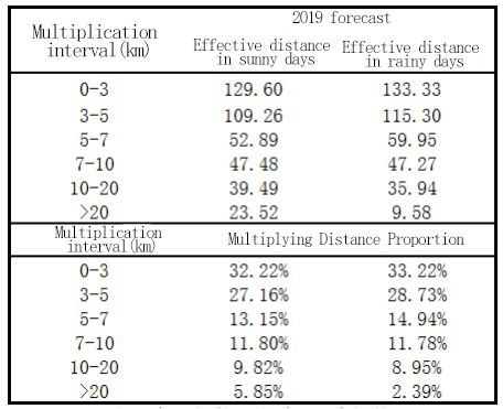
2020 International Conference on Applied Physics and Computing (ICAPC 2020)               IOP Publishing
Journal of Physics: Conference Series            1650 (2020) 032074 doi:10.1088/1742-6596/1650/3/032074

Decision theory analysis of airport driver and management
based on linear regression analysis

                     Jingmin Yao1, Zhenbo Lu2 and Zicheng Wang3
                     1
                       School of Applied Science and Technology, Hainan University, Danzhou, Hainan,
                     571737, China
                     2
                       Marine Engineering College, Dalian Maritime University, Dalian, Liaoning, 116026,
                     China
                     3
                       School of Civil Engineering, Central South University, Changsha, Hunan, 410075,
                     China

                     Abstract. In this paper, we turn the driver decision problem into: the game theory
                     between the revenue generated by the driver after waiting for the waiting in the storage
                     pool and the return to the urban area. When the driver chooses to wait for the yield
                     greater than the return to the urban area, he chooses to wait. On the contrary, we return
                     directly to the urban area. Meanwhile, we collect, analyze and process the information
                     about the taxi in Shanghai Pudong Airport and Shanghai, and calculate the proportion
                     of passengers choosing taxi after arriving at the airport through the Nested Logit model.
                     And multiple linear regression equation model is used to deal with airport passenger
                     throughput, forecast the take-off and landing of flights, speed analysis of taxis and the
                     driving range of taxis under different weather conditions, and ultimately determine the
                     drivers' different decisions.

                     Keywords: taxi drivers, queuing theory, linear regression analysis.

1. Introduction
Since twenty-first Century, with the rapid development of domestic aviation industry and economy,
people have chosen aviation as a convenient mode of transportation. Because of the continuous
development of the aviation industry, the traffic environment and traffic management of the airport area
have higher requirements, and also bring huge passenger traffic to the airport area. Correspondingly, it
has also led to the economic effect of the transportation industry in the region. The promotion of
economic effects has had a huge impact on the competition in various industries, and these competitions
will be reflected in the actual problems faced by some taxi drivers. Therefore, as an important part of
airport traffic, taxis are especially important for passengers to travel reasonably. In addition, taking into
account the principle of carrying passengers at airports. It is not allowed to refuse to load. The
uncertainty of the passenger destination will greatly affect the taxi drivers' income. In order to balance
this difference, the airport needs a reasonable plan to properly regulate taxi drivers to better maintain
airport traffic patency.

              Content from this work may be used under the terms of the Creative Commons Attribution 3.0 licence. Any further distribution
              of this work must maintain attribution to the author(s) and the title of the work, journal citation and DOI.
Published under licence by IOP Publishing Ltd                          1
2020 International Conference on Applied Physics and Computing (ICAPC 2020) IOP Publishing
Journal of Physics: Conference Series 1650 (2020) 032074 doi:10.1088/1742-6596/1650/3/032074
2. The establishment and solution of the first problem model
2.1. Analysis
We can see that the topic is a decision-making problem. We take the driver's income and the number of
airport passengers as the starting point. We consider making a decision by comparing the net income
generated by the two schemes. After analysis, we can see that the net income of PA is the w1 of the
passenger's return to the urban area after waiting. The net income of PB is w2 within the same waiting
time of PA in the urban area, which means that the final decision can be obtained by comparing the
difference between the two incomes and comparing with zero.
2.2. Model establishment
According to the analysis, drivers will make decision analysis on PA and PB, where PA will return to
the urban area after waiting for passengers, and PB will directly return to the urban area.
First, we discuss the choice of PA. At this point, the driver needs to enter the waiting queue. There
are two main factors that affect the waiting queue flow: the number of queued teams and the number of
passengers waiting to get on the bus. As a result of the assumption that the t1 can be landed at the same
time and the number of landing is F, F is directly observed by the driver. That is, F is a fixed value. By
finding data, we can get the average number of passengers per airport of an airport K. and then establish
the Nested LogitModel model to calculate the proportion of taxi passengers after arriving at the airport.
It can be concluded that the number of taxi drivers arriving at a taxi in a certain period of time is as
follows:
L F K (1)
By calculating the occupancy ratio of the taxi passengers, we can see that each vehicle will carry m
passengers on average, that is, the driver needs at least a critical value. The passengers are waiting at the
waiting point. Combined with the arrangements of the airport for the driving points, we can calculate a
reasonable number of vehicles that can be carried away by M. per unit time:
N m (2)
Considering that if the threshold value is greater than the waiting point of the passenger point, that
is, the driver is not able to receive passengers, then it will take an additional t1 time for each occasion.
With the above parameters, the expression of waiting time t can be obtained as follows:
N Nm (3)
t t1
M L
When the driver gets the passengers back to the urban area, assuming that the distance from the
airport to the city centre is fixed at S, the local taxi's charging function is s (the standard of taxi charges
all over the country). PA's income is W1:
W1 (s) (4)
Then we discuss the PB, because the assumption is the same destination, that is, the length of the
airport to the urban area, so the time for PB to work in the urban area is the waiting time in PA. t is not
difficult to find that the profit generated by PB is the profit generated by the drivers in the urban area
during the waiting time in PA. We also call this profit the time cost of PA in the waiting time.
Because we are talking about the actual situation, we can get the current time period. Under the
weather condition, the empty load rate of taxis in the urban area is alpha, the average speed of taxis is
Vt, and the average distance of each taxi is S0.
22020 International Conference on Applied Physics and Computing (ICAPC 2020) IOP Publishing
Journal of Physics: Conference Series 1650 (2020) 032074 doi:10.1088/1742-6596/1650/3/032074
It can be concluded that real load time = total time*(1-no-load rate); real load distance=real load
time*average speed; actual load times=real load distance/average distance; urban profit=real load
frequency*per single income.
Bring the relevant variables to the PB (PA's time cost):
vt
W2 t (1 ) ( S0 ) (5)
S0
Taking all the above into account, in order to facilitate drivers' decision making, the decision decision
of drivers is D.
(6)
2.3. Model solution
In order to make decisions on the two plans, we analyze them by calculating the critical value.
According to the actual situation analysis, the data in the model are positive, that is, in order to
determine the positive and negative of D and make d=0 solve the critical value, the range of the critical
value is analyzed.
Let D=w1 -w2 =0 bring in (4) (5) formula: the actual load times.
s
(7)
( s0 )
That is to say, under the current circumstances, the number of times that can be completed in the
urban area is equal to the ratio of airport to urban income and the average per capita income in the urban
area, the two schemes have the same benefit, and the critical load is a.
The critical number a is introduced into (5) formula.
A S0 (1 )
t (8)
Vt
Where S0/vt is the average time spent per unit, (1- alpha) is the real load rate of the taxi, we can get
the algebraic expression on the right side of the upper form to indicate the time needed to complete the
critical load time A single in the current situation. We note that the time is TL and then TL is brought
into (3):
N
TL t1 (9)
M L
Remember t x t1 the number of passengers who choose to take taxis in the time of arrival is
L
N
exactly enough to accommodate all the waiting vehicles in the pool. t y required for passengers to
M
leave the waiting vehicles in all pools. The total waiting time is t=tx+t y.
Combined with the critical value, we have:
When t>TL, that is, D2020 International Conference on Applied Physics and Computing (ICAPC 2020) IOP Publishing
Journal of Physics: Conference Series 1650 (2020) 032074 doi:10.1088/1742-6596/1650/3/032074
When t=TL, or D=0, the two options yield the same returns.
When T0, PA should be chosen for higher income.
3. Establishment and solution of second problem models
3.1. Analysis
This problem is based on the previous issue. The information collected from Shanghai Pudong Airport
and Shanghai taxi is analyzed and processed, and the proportion of trip mode after arriving at the airport
is calculated through the Nested Logit model. And multiple linear regression equation is used to establish
the relationship between taxi demand and weather factors. By collecting and forecasting information,
the basic traffic parameters of taxi cab can be obtained.
3.2. Model establishment
In this paper, the Nested Logit model is applied to the choice of different modes of transportation,
according to its inherent mechanism, the model of determining the choice tree and determining the mode
of choice is determined, and then the proportion of the taxi choice is predicted. The result can reflect the
waiting time of taxi drivers. A double-layer NL model is established.
According to the theory of Nested Logit model, we can see the probability of a travelers choosing
the mode of trip in I.
PX i a P(i X ) a PXa (10)
Among them, PXia is the probability of a passengers choosing the mode of transportation I; Xi is the
probability of selecting the I of the I under a certain traffic mode. P(i|X)a is the probability of a for
passengers a on the basis of choosing a certain way.
e1 Q( i X ) a
P( i / X ) a N (11)
e Q
i 1
2
(i X ) a
e 2 QXa
PXn 2
e Q
X 1
2
Xa (12)
1 N
QXa Q ' Xa Q *Xa ln exp(1Q *( i X ) a ) (13)
i 1
RX i a Q i X a QXa (i X ) a Xa (14)
Q(i|x)a in formula (11) represents the part of utility changing with X when a passenger selects mode I;
QXa in formula (12) is the effect of a passenger selecting mode I, Q*Xa and Q'Xa are respectively the
part of effect changing with I when a passenger selects mode X, which is independent of I; μ(i|x)a in
formula (14) is the utility probability term of I selection branch when a passenger selects mode X, and
μ(i|X)a is the effect when a passenger selects mode X Using probability term
Then, the maximum likelihood function method is used to estimate the parameters, and the likelihood
function k* is constructed.
42020 International Conference on Applied Physics and Computing (ICAPC 2020) IOP Publishing
Journal of Physics: Conference Series 1650 (2020) 032074 doi:10.1088/1742-6596/1650/3/032074
N Ma Li
K * Pa ( ) ( )a (15)
a 1 m r 1
1, traveler n, select i
( ) n (16)
0, other
The logarithm of the final k* is obtained, and then the maximum value of the formula is obtained to
get the estimated value of the parameter.
3.3. Model solution
Based on the convenience of finding data, we chose Shanghai Pudong International Airport as a practical
problem.
For the solution of the problem, that is to say, under the decision model established by the first
problem, the range or the determined value of all objective variables under different environmental
factors can be solved through a series of processes, and then a lot of simulation analysis is carried out
on the actual situation, and finally the decision plan for the problem is obtained.
3.3.1. Average passenger number k. Because of the development of science and technology and the
increase of people's travel times, we can not simply represent the future data through past data. Therefore,
we can get the predicted model by analyzing the data in recent years by means of linear regression
analysis.
Through information available, the annual passenger throughput and the total number of flights taken
off and landing at Shanghai Pudong Airport in 2004 ~2014.
Considering the scheduling and average state of flights in different months of the year, we think that
passenger throughput / take-off and landing is equal to the average number of passengers on average.
By calculating the average passenger carrying capacity in 2004~2014, we made a linear regression
analysis of the ten sets of data and got the future prediction model (see Table 1).
K 2.3079 105.6 (17)
R2= 0.7869
Table 1. Prediction results and errors
By comparing the predicted and actual values in 2015 ~2018, we found that the error is within the
acceptable range. We think the regression model is reasonable, that is to say, the average number of
passengers carrying k=149.52 passengers in 2019 is acceptable.
3.3.2. Average driving speed of each period V t. Then we discuss the average driving speed of V t in the
urban area. We get the average driving speed of vehicles in different periods of Shanghai and sunny and
rainy days under different conditions. We consider that the average driving speed is less affected by
other factors, and the average speed of each period is the average of the data.
52020 International Conference on Applied Physics and Computing (ICAPC 2020) IOP Publishing
Journal of Physics: Conference Series 1650 (2020) 032074 doi:10.1088/1742-6596/1650/3/032074
3.3.3. Distribution of no-load rate at each time period. Similarly, we have done a lot of data analysis
of the taxi load rate in Shanghai urban area. We find that the idle rate of taxis is entirely dependent on
the distribution of weather and time periods. We do not consider the special circumstances. We believe
that the no-load rate of each period is the arithmetic mean of the set of sets.
3.3.4. Average taxi ride distance under different conditions. We analyzed the average effective distance
of six kinds of multiplying intervals (0-3km; 3-5km; 5-7km; 7-10km; 10-20km; >20km) of two kinds
of weather in Shanghai taxi in 2013 ~2018, and found that the effective distance of each interval
increased significantly with the growth of the year. We can regress the data again to get two kinds of
weather in 2019. The effective distance and multiplying interval of different multiplying distances
account for the proportion of all intervals, as shown in Table 2.
Table 2. Average probability of different distances
Then the average value of the distance interval is Si, and the multiplying distance is Pi, then the
expected distance between the six intervals is:
k
E Si Pi (18)
i 0
By calculating, the average taxi ride distance is 5.39km, and the average taxi ride distance is 4.69km.
In rainy days.
3.3.5. Design simulation experiment. In order to simulate the actual situation reasonably, we set up four
simulation quantities, namely, the weather (sunny and rainy days), the time (24 time periods), the
number of queuing vehicles and the number of landing flights.
Taking into account the need for adequate test data and realistic rationality, the simulation is:
1) The number of queuing vehicles is N = 10*i (i = 0,1,2,3...19)
2) The number of flights per unit time is F = f (f = 0,1,2,3...12)
3) The weather was judged to be 0 or 1 (0 for sunny days; 1 for Yu Tian).
4) The time is t = 0,1,2,3....23
5) The simulation results are obtained after simulation of these simulates.
By analyzing the simulation results,
62020 International Conference on Applied Physics and Computing (ICAPC 2020) IOP Publishing
Journal of Physics: Conference Series 1650 (2020) 032074 doi:10.1088/1742-6596/1650/3/032074
Table 3. Basis for decision making
The final decision is:
Step 1: Drivers get a waiting time of t by passing the observed queuing vehicles and landing flights.
Step 2: Drivers determine whether t is less than 80min.
Step 3: If it is, no matter other factors directly choose to pool car queuing passengers.
Step 3: If not, decisions are made through current time and weather, and make decisions according
to Table3.
References
[1] Designated academic committee, Fuzhou Municipal People's government. Bus priority and
mitigation measures: Proceedings of the 2012 annual conference of China's urban transport
planning and twenty-sixth Academic Symposium [C]. Academic Committee on urban traffic
planning of China Urban Planning Society, Fuzhou Municipal People's Government: China
Urban Planning Association, 2012: 9.
[2] Yao Yanbin, Gao Jinhua. Prediction of Airport Rail Transit on land side traffic diversion [J].
Journal of East China Jiaotong University, 2006 (01): 48-51.
[3] Yuexi exhibition. Airport land side traffic demand forecast and distributed road design [J]. Jilin
University, 2011.
[4] Geng Zhongbo, Song Guohua, Zhao Qi. Research on the comparison of the taxi boarding scheme
of the capital airport based on VISSIM [J]. Journal of Civil Aviation University of China, 2013,
31 (06): 55-59.
[5] Li Yunlong. Feature classification of large aviation hub based on source matrix [J]. Journal of
Chongqing Jiaotong University (SOCIAL SCIENCES), 2017, 17 (03): 42-46.
[6] Liu Xinmeng. Brief analysis on the coordinated development of civil aviation and one-stop travel
platform -- Taking "drop trip" as an example [J]. Traffic accounting, 2017 (05): 70-74.
[7] LU Hong. Prediction of passenger throughput at Shanghai Hongqiao Airport. [J]. modern
business, 2017 (26): 185-186.
[8] Huang Canbin, Yang Xiaoguang, valley Songyuan, Shanghai Hongqiao hub airport passenger
flow characteristics analysis [J]. Traffic and transportation (Academic Edition), 2011 (01):
133-136.
[9] Meng Wei Yan. Application Research of intelligent station technology in airport taxi management.
[A]. China Intelligent Transportation Association.2014 ninth China Intelligent Transportation
72020 International Conference on Applied Physics and Computing (ICAPC 2020) IOP Publishing
Journal of Physics: Conference Series 1650 (2020) 032074 doi:10.1088/1742-6596/1650/3/032074
annual conference conference papers [C]. China Intelligent Transportation Association: China
Intelligent Transportation Association, 2014: 5.
[10] Zhang Lanfang, Bian Tao, Zhang Liang. Selection of large airport connection modes based on
NL model [J]. Urban traffic, 2017, 15 (02): 40-47.
8You can also read